Page 291 - Introduction to Autonomous Mobile Robots

Chapter 6
276
When faced with range sensor data, a popular way of determining rotation direction and
speed is to simply subtract left and right range readings of the robot. The larger the differ-
ence, the faster the robot will turn in the direction of the longer range readings. The follow-
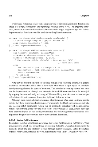
ing two rotation functions could be used for our Bug2 implementation:

private int ComputeGoalSeekRot(angle goalAngle) {
if (Math.abs(goalAngle) < pi/10) return 0;
else return (goalAngle * 100);
} // end ComputeGoalSeekRot() //
private int ComputeRWFRot(sensorvals sonars) {
int minLeft, minRight, desiredTurn;
minRight = MinRange(sonars, -pi/2, 0);
minLeft = MinRange(sonars, 0, pi/2);
if (Math.max(minRight,minLeft) < 200) return (400);
// hard left turn
else {
desiredTurn = (400 - minRight) * 2;
desiredTurn = Math.inttorange(-400, desiredTurn, 400);
return desiredTurn;
} // end else
} // end ComputeRWFRot() //

Note that the rotation function for the case of right wall following combines a general
avoidance of obstacles with a bias to turn right when there is open space on the right,
thereby staying close to the obstacle’s contour. This solution is certainly not the best solu-
tion for implementation of Bug2. For example, the wall follower could do a far better job
by mapping the contour locally and using a PID control loop to achieve and maintain a spe-
cific distance from the contour during the right wall following action.
Although such simple obstacle avoidance algorithms are often used in simple mobile
robots, they have numerous shortcomings. For example, the Bug2 approach does not take
into account robot kinematics, which can be especially important with nonholonomic
robots. Furthermore, since only the most recent sensor values are used, sensor noise can
have a serious impact on real-world performance. The following obstacle avoidance tech-
niques are designed to overcome one or more of these limitations.

6.2.2.2 Vector field histogram
Borenstein, together with Koren, developed the vector field histogram (VFH) [43]. Their
previous work, which was concentrated on potential fields [92], was abandoned due to the
method’s instability and inability to pass through narrow passages. Later, Borenstein,
together with Ulrich, extended the VFH algorithm to yield VFH+ [150] and VFH*[149].