Page 296 - Introduction to Autonomous Mobile Robots

Planning and Navigation

y 281
(x min , y min )
c min
(x , y )
Obstacle obs obs
c max (x max , y max )

x

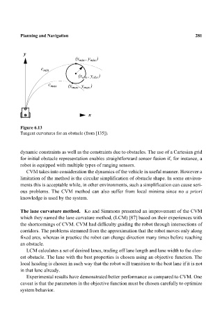
Figure 6.13
Tangent curvatures for an obstacle (from [135]).

dynamic constraints as well as the constraints due to obstacles. The use of a Cartesian grid
for initial obstacle representation enables straightforward sensor fusion if, for instance, a
robot is equipped with multiple types of ranging sensors.
CVM takes into consideration the dynamics of the vehicle in useful manner. However a
limitation of the method is the circular simplification of obstacle shape. In some environ-
ments this is acceptable while, in other environments, such a simplification can cause seri-
ous problems. The CVM method can also suffer from local minima since no a priori
knowledge is used by the system.

The lane curvature method. Ko and Simmons presented an improvement of the CVM
which they named the lane curvature method, (LCM) [87] based on their experiences with
the shortcomings of CVM. CVM had difficulty guiding the robot through intersections of
corridors. The problems stemmed from the approximation that the robot moves only along
fixed arcs, whereas in practice the robot can change direction many times before reaching
an obstacle.
LCM calculates a set of desired lanes, trading off lane length and lane width to the clos-
est obstacle. The lane with the best properties is chosen using an objective function. The
local heading is chosen in such way that the robot will transition to the best lane if it is not
in that lane already.
Experimental results have demonstrated better performance as compared to CVM. One
caveat is that the parameters in the objective function must be chosen carefully to optimize
system behavior.