Page 297 - Introduction to Autonomous Mobile Robots

282

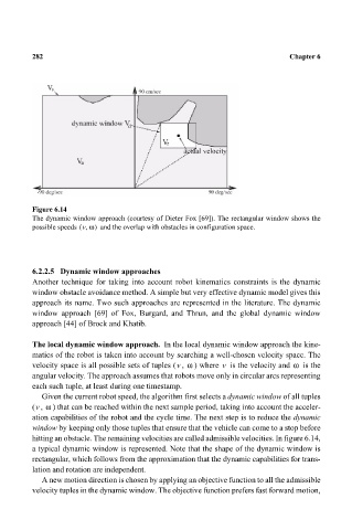
Figure 6.14 Chapter 6
The dynamic window approach (courtesy of Dieter Fox [69]). The rectangular window shows the
possible speeds v ω,( ) and the overlap with obstacles in configuration space.

6.2.2.5 Dynamic window approaches
Another technique for taking into account robot kinematics constraints is the dynamic
window obstacle avoidance method. A simple but very effective dynamic model gives this
approach its name. Two such approaches are represented in the literature. The dynamic
window approach [69] of Fox, Burgard, and Thrun, and the global dynamic window
approach [44] of Brock and Khatib.

The local dynamic window approach. In the local dynamic window approach the kine-
matics of the robot is taken into account by searching a well-chosen velocity space. The
velocity space is all possible sets of tuples ( , ω ) where is the velocity and ω is the
v
v
angular velocity. The approach assumes that robots move only in circular arcs representing
each such tuple, at least during one timestamp.
Given the current robot speed, the algorithm first selects a dynamic window of all tuples
v ω
(, ) that can be reached within the next sample period, taking into account the acceler-
ation capabilities of the robot and the cycle time. The next step is to reduce the dynamic
window by keeping only those tuples that ensure that the vehicle can come to a stop before
hitting an obstacle. The remaining velocities are called admissible velocities. In figure 6.14,
a typical dynamic window is represented. Note that the shape of the dynamic window is
rectangular, which follows from the approximation that the dynamic capabilities for trans-
lation and rotation are independent.
A new motion direction is chosen by applying an objective function to all the admissible
velocity tuples in the dynamic window. The objective function prefers fast forward motion,