Page 80 - Introduction to Autonomous Mobile Robots

Mobile Robot Kinematics

Y R 65

v y1
ω 1 1
v
x1 X R
2
⋅
3 r ϕ
1
ICR
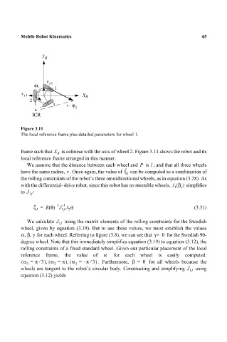
Figure 3.11
The local reference frame plus detailed parameters for wheel 1.

frame such that X is colinear with the axis of wheel 2. Figure 3.11 shows the robot and its
R
local reference frame arranged in this manner.
We assume that the distance between each wheel and is , and that all three wheels
P
l
have the same radius, . Once again, the value of ξ · can be computed as a combination of
r
I
the rolling constraints of the robot’s three omnidirectional wheels, as in equation (3.28). As
with the differential- drive robot, since this robot has no steerable wheels, J β() simplifies
1 s
to J 1f :
· – 1 – 1
ξ = R θ() J J ϕ · (3.31)
I 1f 2
We calculate J 1f using the matrix elements of the rolling constraints for the Swedish
wheel, given by equation (3.19). But to use these values, we must establish the values
α βγ for each wheel. Referring to figure (3.8), we can see that γ= 0 for the Swedish 90-
,,
degree wheel. Note that this immediately simplifies equation (3.19) to equation (3.12), the
rolling constraints of a fixed standard wheel. Given our particular placement of the local
reference frame, the value of α for each wheel is easily computed:
⁄
⁄
(
( α = π 3) α = π) α = – π 3) . Furthermore, β = 0 for all wheels because the
(
,
,
1 2 3
wheels are tangent to the robot’s circular body. Constructing and simplifying J 1f using
equation (3.12) yields