Page 79 - Introduction to Autonomous Mobile Robots

64

Y I Chapter 3

v(t)
ω(t) θ

X I

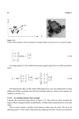
Figure 3.10
A three-wheel omnidrive robot developed by Carnegie Mellon University (www.cs.cmu.edu/~pprk).

10 l
· J ϕ
2
10 l R θ()ξ = (3.29)
–
I
0
010
Inverting equation (3.29) yields the kinematic equation specific to our differential drive
robot:

1 1
– 1 --- ---0
10 l 2 2
· – 1 J ϕ – 1 J ϕ
2
2
ξ = R θ() 10 l = R θ() 0 0 1 (3.30)
–
I
0 0
01 0 1 1
–
----- ----- 0
2l 2l
This demonstrates that, for the simple differential-drive case, the combination of wheel
rolling and sliding constraints describes the kinematic behavior, based on our manual cal-
culation in section 3.2.2.
3.2.5.2 An omnidirectional robot example
Consider the omniwheel robot shown in figure 3.10. This robot has three Swedish 90-
degree wheels, arranged radially symmetrically, with the rollers perpendicular to each main
wheel.
First we must impose a specific local reference frame upon the robot. We do so by
choosing point at the center of the robot, then aligning the robot with the local reference
P