Page 131 - Introduction to Computational Fluid Dynamics

P1: IWV
12:28
May 20, 2005
0 521 85326 5
0521853265c05
CB908/Date
110
∆X 1w ∆X 1e 2D CONVECTION – CARTESIAN GRIDS
∆X 1ee
N Ne NE
n ne
∆X
2n
W w P e E ee EE
∆X 2

s se
∆ ∆X 2s

S Se SE

∆X 1
Nodes Cell Faces
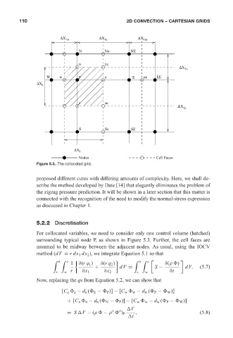
Figure 5.3. The collocated grid.

proposed different cures with differing amounts of complexity. Here, we shall de-
scribe the method developed by Date [14] that elegantly eliminates the problem of
the zigzag pressure prediction. It will be shown in a later section that this matter is
connected with the recognition of the need to modify the normal-stress expression
as discussed in Chapter 1.

5.2.2 Discretisation

For collocated variables, we need to consider only one control volume (hatched)
surrounding typical node P, as shown in Figure 5.3. Further, the cell faces are
assumed to be midway between the adjacent nodes. As usual, using the IOCV
method (dV = rdx 1 dx 2 ), we integrate Equation 5.1 so that

n e
n e
1 ∂(rq 1 ) ∂(rq 2 ) ∂(ρ )
+ dV = S − dV. (5.7)
s w r ∂x 1 ∂x 2 s w ∂t
Now, replacing the qs from Equation 5.2, we can show that

[C e e − d e ( E − P )] − [C w w − d w ( P − W )]
+ [C n n − d n ( N − P )] − [C w w − d w ( P − W )]

V
o o
= S V − (ρ − ρ ) P , (5.8)
t