Page 127 - Introduction to Computational Fluid Dynamics

P1: IWV
May 20, 2005
12:28
CB908/Date
0521853265c05
106
WALL
X 2 0 521 85326 5 2D CONVECTION – CARTESIAN GRIDS
X 1 RECIRCULATION
EXIT
INFLOW
r SYMMETRY

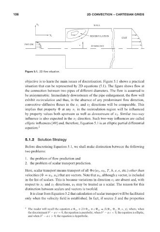
Figure 5.1. 2D flow situation.

objective is to learn the main issues of discretisation. Figure 5.1 shows a practical
situation that can be represented by 2D equations (5.1). The figure shows flow at
the connection between two pipes of different diameters. The flow is assumed to
be axisymmetric. Immediately downstream of the pipe enlargement, the flow will
exhibit recirculation and thus, in the absence of any predominant flow direction,
convective–diffusive fluxes in the x 1 and x 2 directions will be comparable. This
implies that property at any x 1 in the recirculation region will be influenced
by property values both upstream as well as downstream of x 1 . Similar two-way
influence is also expected in the x 2 direction. Such two-way influences are called
elliptic influences [49] and, therefore, Equation 5.1 is an elliptic partial differential
equation. 2

5.1.2 Solution Strategy

Before discretising Equation 5.1, we shall make distinction between the following
two problems:
1. the problem of flow prediction and
2. the problem of scalar transport prediction.

Here, scalar transport means transport of all s(u 3 , ω k , T , h, e, , etc.) other than
velocities ( = u 1 , u 2 ) that are vectors. Note that u 3 , although a vector, is included
in the list of scalars. This is because variations in direction x 3 are absent and, with
respect to x 1 and x 2 directions, u 3 may be treated as a scalar. The reason for this
distinction between scalars and vectors is twofold.
It is clear from Equation 5.2 that calculation of scalar transport will be facilitated
only when the velocity field is established. In fact, if source S and the properties

2 The reader will recall the equation a xx + 2 b xy + c yy = S ( x , y , , x, y), where, when
2
2
the discriminant b − ac = 0, the equation is parabolic; when b − ac < 0, the equation is elliptic;
2
and when b − ac > 0, the equation is hyperbolic.