Page 122 - Introduction to Computational Fluid Dynamics

P1: IWV
0 521 85326 5
CB908/Date
0521853265c04
EXERCISES
(b)
(a) May 25, 2005 11:7 101
30 30
Re = 3000 Re = 10000
20 COMPUTED U + 20 COMPUTED U +

U + U +
+
U = 2.5 ln Y +
U = 2.5 ln Y + 5.5 + 5.5
10
10
+ +
U = Y + +
U = Y
Re t
Re t
0
1 10 + 100 1 10 + 100
Y Y
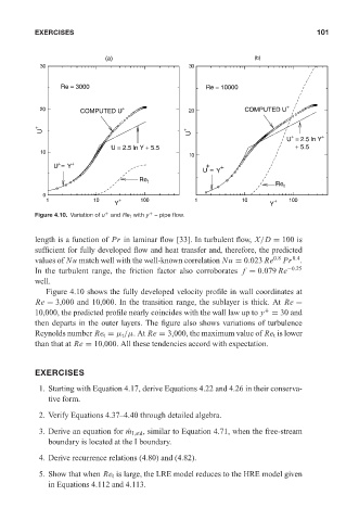
Figure 4.10. Variation of u and Re t with y – pipe flow.
+
+
length is a function of Pr in laminar flow [33]. In turbulent flow, X/D = 100 is
sufficient for fully developed flow and heat transfer and, therefore, the predicted
values of Nu match well with the well-known correlation Nu = 0.023 Re 0.8 Pr 0.4 .
In the turbulent range, the friction factor also corroborates f = 0.079 Re −0.25
well.
Figure 4.10 shows the fully developed velocity profile in wall coordinates at
Re = 3,000 and 10,000. In the transition range, the sublayer is thick. At Re =
10,000, the predicted profile nearly coincides with the wall law up to y = 30 and
+
then departs in the outer layers. The figure also shows variations of turbulence
Reynolds number Re t = µ t /µ.At Re = 3,000, the maximum value of Re t is lower
than that at Re = 10,000. All these tendencies accord with expectation.

EXERCISES

1. Starting with Equation 4.17, derive Equations 4.22 and 4.26 in their conserva-
tive form.
2. Verify Equations 4.37–4.40 through detailed algebra.

3. Derive an equation for ˙ m I,std , similar to Equation 4.71, when the free-stream
boundary is located at the I boundary.
4. Derive recurrence relations (4.80) and (4.82).

5. Show that when Re t is large, the LRE model reduces to the HRE model given
in Equations 4.112 and 4.113.