Page 129 - Introduction to Computational Fluid Dynamics

P1: IWV
May 20, 2005
0 521 85326 5
12:28
0521853265c05
CB908/Date
108
N 2D CONVECTION – CARTESIAN GRIDS
nW nw n ne

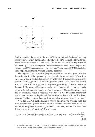
Figure 5.2. The staggered grid.
U f1
W w P e E

sW sw s U f2 se

wS S eS

Such an equation, however, can be derived from explicit satisfaction of the mass
conservation equation. In the sections to follow, the SIMPLE method for determi-
nation of the pressure field is presented. This method was developed by Patankar
and Spalding [51]. It is among the most extensively used methods in CFD practice.
In fact, most CFD packages employ this method. The acronym SIMPLE stands for
Semi-Implicit Method for Pressure-Linked Equations. 3
The original SIMPLE method [51] was derived for Cartesian grids in which
the scalar s (including pressure p) and the velocity vectors were defined in a
staggered arrangement (see Figure 5.2). To understand this arrangement, consider
typical node P (i, j) with the surrounding control volume whose faces are located
at e, w, n, and s. In the staggered arrangement, pressure p i, j is stored/defined at
the node P. The same holds for other scalars i, j . However, the vector u f1 (i, j)is
stored at the cell face w and vector u f2 (i, j) is stored at cell face s. Thus, the vectors
and the scalars are stored in staggered locations. It is easy to identify appropriate
control volumes surrounding the cell-face locations as shown in Figure 5.2. Thus,
in the (i, j) address system, there are three partially overlapping control volumes.
Now, the SIMPLE method requires that to determine the pressure field, the
mass conservation equation must be satisfied over the control volume (ne-se-sw-
nw) surrounding node P where p i, j is stored. Thus, using the IOCV method, the
discretised version of Equation 5.3 is written as

V

o
[(ρ ru f1 ) e − (ρ ru f1 ) w ] x 2 + [(ρ ru f2 ) n − (ρ ru f2 ) s ] x 1 =− ρ P − ρ ,
P
t
(5.6)

3 In compressible flows, p = ρ R g T , where R g is the gas constant, must be added to the equation
set (5.3–5.6). This equation of state is used to determine density ρ.