Page 138 - Introduction to Computational Fluid Dynamics

P1: IWV
CB908/Date
0 521 85326 5
0521853265c05
5.2 SIMPLE – COLLOCATED GRIDS
one-dimensional averaging as May 20, 2005 12:28 117
u
AP uf1 = 1
AP + AP u ,
e P E
2
u
AP uf2 = 1
AP + AP u , (5.52)
n P N
2
u
where AP = AP u 1 = AP u 2 on collocated grids.
These derivations show that Equations 5.30 and 5.31 can be replaced by Equa-
tions 5.34 and 5.51, respectively. Thus, the mass-conserving pressure-correction
equation (5.25) can be effectively written as

1 ∂ ρ l+1 r α V ∂p m
1 ∂ ρ l+1 r α V ∂p m
+
r ∂x 1 AP u f1 ∂x 1 r ∂x 2 AP u f2 ∂x 2
∂(ρ) 1 ∂ l+1 l 1 ∂ l+1 l
= + r ρ u 1 + r ρ u 2
∂t r ∂x 1 r ∂x 2
l+1
l+1
1 ∂ ρ r α V ∂p sm 1 ∂ ρ r α V ∂p sm
− + .
r ∂x 1 AP u f1 ∂x 1 r ∂x 2 AP u f2 ∂x 2
(5.53)

This equation represents the appropriate form of the mass-conserving pressure-
correction equation on collocated grids.

5.2.4 Further Simplification

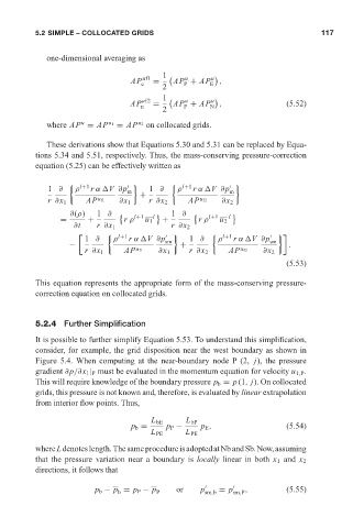
It is possible to further simplify Equation 5.53. To understand this simplification,
consider, for example, the grid disposition near the west boundary as shown in
Figure 5.4. When computing at the near-boundary node P (2, j), the pressure
gradient ∂p/∂x 1 | P must be evaluated in the momentum equation for velocity u 1,P .
This will require knowledge of the boundary pressure p b = p (1, j). On collocated
grids, this pressure is not known and, therefore, is evaluated by linear extrapolation
from interior flow points. Thus,

L bE L bP
p b = p P − p E , (5.54)
L PE L PE
whereLdenoteslength.ThesameprocedureisadoptedatNbandSb.Now,assuming
that the pressure variation near a boundary is locally linear in both x 1 and x 2
directions, it follows that

p b − p = p P − p P or p sm,b = p sm,P , (5.55)
b