Page 139 - Introduction to Computational Fluid Dynamics

P1: IWV
12:28
May 20, 2005
0 521 85326 5
0521853265c05
CB908/Date
118
N 2, j + 1 2D CONVECTION – CARTESIAN GRIDS
Nb
q
1, j
1, j P 2, j 3, j
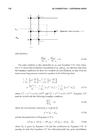
b Figure 5.4. West boundary, i = 1.
E
Φ
θ S
Sb
2, j − 1

i = 1

and, therefore,

∂p ∂p
= sm = 0. (5.56)
sm
∂x 1 ∂n
b b

The same condition is also applicable to p (see Equation 5.33). Now, Equa-
m
tion 5.53 shows that multipliers of gradients of p and p are identical and, since

m sm
the boundary conditions for these two variables are also identical, we may write the
mass-conserving pressure correction equation in the following form:

1 ∂ p ∂p 1 ∂ p ∂p

1 +
2
r ∂x 1 ∂x 1 r ∂x 2 ∂x 2
∂(ρ l+1 ) 1 ∂ l+1 l 1 ∂ l+1 l
= + r ρ u 1 + r ρ u 2 , (5.57)
∂t r ∂x 1 r ∂x 2
p l+1 uf1 p l+1 uf2
where
= ρ r α V/AP and
= ρ r α V/AP . Equation 5.57
1 2
must be solved with the following boundary condition:

∂p
= 0, (5.58)

∂n
b
where the total pressure correction p is given by

p = p + p , (5.59)
m sm
and the discretised form of Equation 5.57 is

AP p = AE p + AW p + AN p + AS p − ˙ m P , (5.60)

S
N
P
E
W
where ˙ m P is given by Equation 5.34 and the coefficients by Equation 5.29. In
passing we note that Equation 5.57 for collocated grids has great resemblance