Page 25 - Introduction to Computational Fluid Dynamics

P2: IWV
P1: JYD/GKJ
CB908/Date
0 521 85326 5
0521853265c01
4
INTRODUCTION
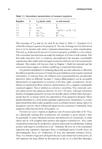
Table 1.1: Generalised representation of transport equations. May 20, 2005 12:20
Equation Φ Γ eff (exch. coef.) S Φ (net source)
1.1 1 0 0
1.2 ω k ρ m D eff R k
1.3 u i µ eff −∂p/∂x i + ρ m B i + S u i
1.4 h k eff / C pm Q
1.5 T k eff / C pm Q / C pm

The meanings of
eff and S for each are listed in Table 1.1. Equation 1.6 is
called the transport equation for property . The rate of change (or time derivative)
term is to be invoked only when a transient phenomenon is under consideration.
The term ρ m denotes the amount of extensive property available in a unit volume.
The convection (second) term accounts for transport of due to bulk motion. This
first-order derivative term is relatively uncomplicated but assumes considerable
significance when stable and convergent numerical solutions are to be economically
obtained. This matter will become clear in Chapter 3. Both the transient and the
convection terms require no further modelling or empirical information.
The greatest impediment to obtaining physically accurate solutions is offered by
the diffusion and the net source (S) terms because both these terms require empirical
information. In laminar flows, the diffusion term represented by the second-order
derivative offers no difficulty because
, being a fluid property, can be accurately
determined (via experiments) in isolation of the flow under consideration. In tur-
bulent (or transitional) flows, however, determination of
eff requires considerable
empirical support. This is labelled as turbulence modelling. This extremely com-
plex phenomenon has attracted attention for over 150 years. Although turbulence
models of adequate generality (at least, for specific classes of flows) have been pro-
posed, they by no means satisfy the expectations of an equipment designer. These
models determine
eff from simple algebraic empirical laws. Sometimes,
eff is also
determined from other scalar quantities (such as turbulent kinetic energy and/or its
dissipation rate) for which differential equations are constituted. Fortunately, these
equations often have the form of Equation 1.6.
The term net source implies an algebraic sum of sources and sinks of . Thus,
in a chemically reacting flow (combustion, for example), a given species k may
be generated via some chemical reactions and destroyed (or consumed) via some
others and R k will comprise both positive and negative contributions. Also, some
chemical reactions may be exothermic, whereas others may be endothermic, making
positive and negative contributions to Q . Similarly, the term B i in the momentum

equations may represent a buoyancy force, a centrifugal and/or Coriolis force, an
electromagnetic force, etc. Sometimes, B i may also represent resistance forces.

Thus, in a mixture of gas and solid particles (as in pulverised fuel combustion), B i
will represent the drag offered by the particles on air, or, in a fluid flow through a