Page 29 - Introduction to Computational Fluid Dynamics

P2: IWV
P1: JYD/GKJ
May 20, 2005
0 521 85326 5
CB908/Date
0521853265c01
8
INTRODUCTION
CARTESIAN 12:20

CURVILINEAR

UNSTRUCTURED

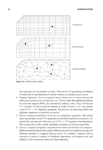
Figure 1.2. Different types of grids.

have polygons of any number of sides. This activity of specifying coordinates
of nodes and of specification of control volumes is called grid generation.
4. Integrate Equation 1.6 over a typical control volume so as to convert the partial
differential equation into an algebraic one. This is unlike the analytical solutions
in which the original PDEs are converted to ordinary ones. Thus, if there are
NV variables of interest and the number of nodes chosen is NP, one obtains
a set of NV × NP algebraic equations. The process of converting PDEs into
algebraic equations is called discretisation.
5. Devise a numerical method to solve the set of algebraic equations. This can be
done sequentially, so that NP equations are solved for each in succession. Al-
ternatively, one may solve the entire set of NV × NP equations simultaneously.
The construction of the overall calculation sequence is called an algorithm.
6. Devise a computer program to implement the numerical method on a computer.
Different numerical methods require different amounts of computer storage and
different amounts of computer time to arrive at a solution. Aspects such as
economy in terms of number of arithmetic operations, convergence rate, and
stability of the numerical method are thus important.