Page 32 - Introduction to Computational Fluid Dynamics

P2: IWV
P1: JYD/GKJ
0 521 85326 5
CB908/Date
0521853265c01
1.5 A NOTE ON NAVIER–STOKES EQUATIONS
TRUE VARIATION May 20, 2005 12:20 11
Y
OF PRESSURE
p
P
X
p
E
p
W
p
P
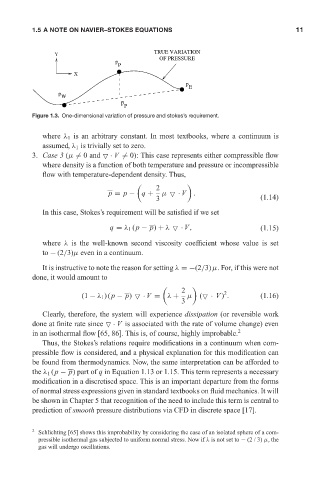
Figure 1.3. One-dimensional variation of pressure and stokes’s requirement.
where λ 1 is an arbitrary constant. In most textbooks, where a continuum is
assumed, λ 1 is trivially set to zero.
3. Case 3 (µ = 0 and · V = 0): This case represents either compressible flow
where density is a function of both temperature and pressure or incompressible
flow with temperature-dependent density. Thus,
2

p = p − q + µ · V .
3 (1.14)
In this case, Stokes’s requirement will be satisfied if we set

q = λ 1 (p − p) + λ · V, (1.15)

where λ is the well-known second viscosity coefficient whose value is set
to − (2/3)µ even in a continuum.
It is instructive to note the reason for setting λ =−(2/3)µ. For, if this were not
done, it would amount to

2 2
(1 − λ 1 )(p − p) · V = λ + µ ( · V ) . (1.16)
3
Clearly, therefore, the system will experience dissipation (or reversible work
done at finite rate since · V is associated with the rate of volume change) even
in an isothermal flow [65, 86]. This is, of course, highly improbable. 2
Thus, the Stokes’s relations require modifications in a continuum when com-
pressible flow is considered, and a physical explanation for this modification can
be found from thermodynamics. Now, the same interpretation can be afforded to
the λ 1 (p − p) part of q in Equation 1.13 or 1.15. This term represents a necessary
modification in a discretised space. This is an important departure from the forms
of normal stress expressions given in standard textbooks on fluid mechanics. It will
be shown in Chapter 5 that recognition of the need to include this term is central to
prediction of smooth pressure distributions via CFD in discrete space [17].

2 Schlichting [65] shows this improbability by considering the case of an isolated sphere of a com-
pressible isothermal gas subjected to uniform normal stress. Now if λ is not set to − (2/3) µ, the
gas will undergo oscillations.