Page 35 - Introduction to Computational Fluid Dynamics

P2: IWV
P1: JYD/GKJ
CB908/Date
0 521 85326 5
0521853265c01
14
INTRODUCTION
. May 20, 2005 12:20
N w q w W ext
INLET
A
τ w
∆ X
X
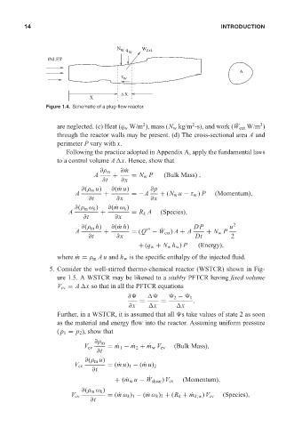
Figure 1.4. Schematic of a plug-flow reactor.
2
3
2
˙
are neglected. (c) Heat (q w W/m ), mass (N w kg/m -s), and work (W ext W/m )
through the reactor walls may be present. (d) The cross-sectional area A and
perimeter P vary with x.
Following the practice adopted in Appendix A, apply the fundamental laws
to a control volume A x. Hence, show that
∂ ˙ m
∂ρ m
A + = N w P (Bulk Mass) ,
∂t ∂x
∂(ρ m u) ∂( ˙ mu) ∂p
A + =−A + (N w u − τ w ) P (Momentum),
∂t ∂x ∂x
∂(ρ m ω k ) ∂( ˙ m ω k )
A + = R k A (Species),
∂t ∂x
∂(ρ m h) ∂( ˙ mh) DP u 2
˙

A + = (Q − W ext ) A + A + N w P
∂t ∂x Dt 2
+ (q w + N w h w ) P (Energy),
where ˙ m = ρ m Au and h w is the specific enthalpy of the injected fluid.

5. Consider the well-stirred thermo-chemical reactor (WSTCR) shown in Fig-
ure 1.5. A WSTCR may be likened to a stubby PFTCR having fixed volume
V cv = A x so that in all the PFTCR equations
∂ 2 − 1
= = .
∂x x x
Further, in a WSTCR, it is assumed that all s take values of state 2 as soon
as the material and energy flow into the reactor. Assuming uniform pressure
( p 1 = p 2 ), show that
∂ρ m
V cv = ˙ m 1 − ˙ m 2 + ˙ m w V cv (Bulk Mass),
∂t
∂(ρ m u)
V cv = ( ˙ mu) 1 − ( ˙ mu) 2
∂t
˙
+ ( ˙ m w u − W shear ) V cv (Momentum),
∂(ρ m ω k )
V cv = ( ˙ m ω k ) 1 − ( ˙ m ω k ) 2 + (R k + ˙ m k,w ) V cv (Species),
∂t