Page 39 - Introduction to Computational Fluid Dynamics

P1: IWV/ICD
0 521 85326 5
10:49
May 25, 2005
0521853265c02
CB908/Date
18
L 1D HEAT CONDUCTION
Q x Q x + x A
∆

x

∆ x

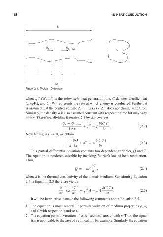
Figure 2.1. Typical 1D domain.

3

where q (W/m ) is the volumetric heat generation rate, C denotes specific heat
(J/kg-K), and Q (W) represents the rate at which energy is conducted. Further, it
is assumed that the control volume V = A (x) × x does not change with time.
Similarly, the density ρ is also assumed constant with respect to time but may vary
with x. Therefore, dividing Equation 2.1 by V ,weget

Q x − Q x+ x ∂(CT )
+ q = ρ . (2.2)

A x ∂t
Now, letting x → 0, we obtain
1 ∂ Q ∂(CT )

− + q = ρ . (2.3)
A ∂x ∂t
This partial differential equation contains two dependent variables, Q and T.
The equation is rendered solvable by invoking Fourier’s law of heat conduction.
Thus,
∂T
Q =−kA , (2.4)
∂x
where k is the thermal conductivity of the domain medium. Substituting Equation
2.4 in Equation 2.3 therefore yields

∂ ∂T ∂(CT )

kA + q A = ρ A . (2.5)
∂x ∂x ∂t
It will be instructive to make the following comments about Equation 2.5.

1. The equation is most general. It permits variation of medium properties ρ, k,
and C with respect to x and/or t.
2. The equation permits variation of cross-sectional area A with x. Thus, the equa-
tion is applicable to the case of a conical fin, for example. Similarly, the equation