Page 41 - Introduction to Computational Fluid Dynamics

P1: IWV/ICD
0 521 85326 5
May 25, 2005
10:49
0521853265c02
CB908/Date
20

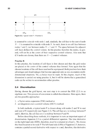
Figure 2.3. Typical node P – Practise A. 1D HEAT CONDUCTION

is assumed to coincide with node 1 and, similarly, the cell face to the east of node
N − 1 is assumed to coincide with node N. As such, there is no cell face between
nodes 1 and 2, nor between nodes N − 1 and N. The space between the adjacent
cell faces defines the control volume. In this practise therefore the nodes, in gen-
eral, will not be at the centre of their respective control volumes. Also note that
if N nodes are chosen, then there are N − 2 control volumes.

Practise B
In this practise, the location of cell faces is first chosen and then the grid nodes
are placed at the centre of the control volumes thus formed. Note again that the
chosen locations of the cell faces need not be equispaced. Both practises have their
advantages and disadvantages that become apparent only as one encounters multi-
dimensional situations. Yet, a choice must be made. In this chapter, much of the
discussion is carried out using practise A, but it will be shown that a generalised
code can be written to accommodate either practise.

2.4 Discretisation

Having chosen the grid layout, our next step is to convert the PDE (2.5) to an
algebraic one. This process of conversion is called discretisation. Here again, there
are two possible approaches:
1. a Taylor series expansion (TSE) method or
2. an integration over a control volume (IOCV) method.

In both methods, a typical node P is chosen along with nodes E and W to east
and west of P, respectively (see Figure 2.3). The cell face at e is midway between P
and E, likewise, the cell face at w is midway between P and W.
Before describing these methods, it is important to note an important aspect of
discretisation. Equation 2.5 is a partial differential equation. The time derivative
on the right-hand side (RHS), therefore, must be evaluated at a fixed x. We choose
this fixed location to be node P. The left-hand side (LHS) of Equation 2.5, however,
contains a partial second derivative with respect to x and, therefore, this derivative