Page 46 - Introduction to Computational Fluid Dynamics

P1: IWV/ICD
CB908/Date
0521853265c02
2.5 STABILITY AND CONVERGENCE
t + ∆t 0 521 85326 5 NEW May 25, 2005 10:49 25

t OLD
i − 1 i i + 1
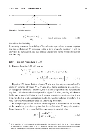
Figure 2.4. Explicit procedure.

ψ [|AE i |+|AW i |]
< 1 for at least one node. (2.30)
|AP i |
Condition for Stability
In unsteady problems, the stability of the calculation procedure, however, requires
o
3
that the coefficient of T contained in the S i term always be positive. It will be
i
shown in the next section that this implies a restriction on the permissible size of
the time step.

2.5.1 Explicit Procedure ψ = 0

In this case, Equation 2.28 will read as
ρ V i C
n
i T i = AE i T o + AW i T o + q ,o A i x
t i+1 i−1 i
o
ρ V i C i o
+ − (AE i + AW i ) T . (2.31)
i
t
Equation 2.31 shows that the values of T i at a new time step are now calculable
o
o
o
explicitly in terms of values T i−1 , T , and T i+1 . Terms containing T i+1 and T i−1
i
do not appear on the RHS. Therefore, the equation is explicit and no iterations are
required. This situation is also depicted in Figure 2.4. Thus, starting with known
initial temperature distribution at t = 0, one can evaluate temperatures at each new
time step. Such a solution procedure is called a marching solution procedure. It is
very easy to devise computer code for a marching procedure.
In an explicit procedure, the issue of convergence is irrelevant but the stability
o
of the calculation procedure requires that the coefficient of T always be positive.
i
From Equation 2.31 it is clear that this requirement is satisfied when
ρ V i C
o
t < i . (2.32)
AE i + AW i
min

3 This condition of positiveness is strictly meant for the case of ψ = 0. For ψ = 1, the condition
is automatically satisfied. For 0 <ψ < 1, however, the condition again holds but can be violated
without impairing stability of the solution procedure. This is discussed in Section 2.5.2.