Page 51 - Introduction to Computational Fluid Dynamics

P1: IWV/ICD
0 521 85326 5
May 25, 2005
10:49
0521853265c02
CB908/Date
30
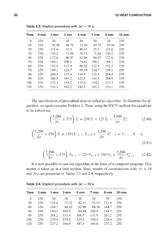
Table 2.3: Implicit procedure with ∆t = 10 s. 1D HEAT CONDUCTION
Time 0 mm 1 mm 3 mm 5 mm 7 mm 9 mm 10 mm
0 250 30 30 30 30 30 250
10 250 92.96 40.79 33.50 40.79 92.96 250
20 250 131.6 55.5 40.65 55.5 131.6 250
30 250 156.2 71.04 50.51 71.04 156.2 250
40 250 172.6 86.07 62.06 86.07 172.6 250
50 250 184.1 100.1 74.41 100.1 184.1 250
60 250 192.5 112.9 86.92 112.9 192.5 250
70 250 199.1 124.7 99.19 124.7 199.1 250
80 250 204.4 135.4 110.9 135.4 204.4 250
90 250 208.9 145.2 122.1 145.2 208.9 250
100 250 213.3 154.2 132.0 154.2 213.3 250
110 250 216.1 162.2 142.1 162.2 216.1 250

The specification of procedural steps is called an algorithm. To illustrate the al-
gorithm, we again consider Problem 1. Then, using the IOCV method, the equations
to be solved are

5,200 5,200 o
+ 375 T 2 = 250 T 1 + 125 T 3 + T , (2.40)
2
t t

5,200 5,200 o
+ 250 T i = 125(T i−1 + T i+1 ) + T i i = 3,..., N − 2,
t t
(2.41)

5,200 5,200 o
+ 375 T N−1 = 125 T N−2 + 250 T N + T N−1 . (2.42)
t t
It is now possible to cast our algorithm in the form of a computer program. This
matter is taken up in a later section. Here, results of computations with t = 10
and 20 s are presented in Tables 2.3 and 2.4, respectively.

Table 2.4: Implicit procedure with ∆t = 20 s.

Time 0 mm 1 mm 3 mm 5 mm 7 mm 9 mm 10 mm
0 250 30 30 30 30 30 250
20 250 121.6 55.52 42.51 55.52 121.6 250
40 250 164.7 84.10 62.90 84.10 164.7 250
60 250 184.5 109.9 84.94 109.9 184.5 250
80 250 201.2 131.9 108.5 131.9 201.2 250
100 250 210.4 150.4 129.1 150.4 210.4 250
120 250 217.2 166.0 147.1 166.0 217.2 250