Page 50 - Introduction to Computational Fluid Dynamics

P1: IWV/ICD
0521853265c02
2.5 STABILITY AND CONVERGENCE
t + CB908/Date 0 521 85326 5 NEW May 25, 2005 10:49 29
∆t

t OLD
i − 1 i i + 1
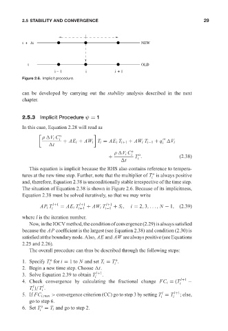
Figure 2.6. Implicit procedure.

can be developed by carrying out the stability analysis described in the next
chapter.

2.5.3 Implicit Procedure ψ = 1
In this case, Equation 2.28 will read as

ρ V i C
n
i
+ AE i + AW i T i = AE i T i+1 + AW i T i−1 + q V i
i
t
ρ V i C i o o
+ T . (2.38)
i
t
This equation is implicit because the RHS also contains reference to tempera-
o
tures at the new time step. Further, note that the multiplier of T is always positive
i
and, therefore, Equation 2.38 is unconditionally stable irrespective of the time step.
The situation of Equation 2.38 is shown in Figure 2.6. Because of its implicitness,
Equation 2.38 must be solved iteratively, so that we may write
AP i T l+1 = AE i T l+1 + AW i T l+1 + S i , i = 2, 3,..., N − 1, (2.39)
i i+1 i−1
where l is the iteration number.
Now, in the IOCV method, the condition of convergence (2.29) is always satisfied
because the AP coefficient is the largest (see Equation 2.38) and condition (2.30) is
satisfied at the boundary node. Also, AE and AW are always positive (see Equations
2.25 and 2.26).
The overall procedure can thus be described through the following steps:
o
o
1. Specify T for i = 1to N and set T i = T .
i i
2. Begin a new time step. Choose t.
3. Solve Equation 2.39 to obtain T l+1 .
i
4. Check convergence by calculating the fractional change FC i = (T l+1 −
i
l
l
T )/T .
i i
l
5. If FC i,max > convergence criterion (CC) go to step 3 by setting T = T l+1 ; else,
i i
go to step 6.
o
6. Set T = T i and go to step 2.
i