Page 55 - Introduction to Computational Fluid Dynamics

P1: IWV/ICD
10:49
May 25, 2005
0 521 85326 5
CB908/Date
0521853265c02
34
MATERIAL K 1 MATERIAL K 2 1D HEAT CONDUCTION
T
i − 1 i i + 1 i i + 1/2 i + 1

i + 1/2
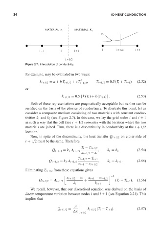
Figure 2.7. Interpolation of conductivity.

for example, may be evaluated in two ways:

k i+1/2 = a + bT i+1/2 + cT 2 , T i+1/2 = 0.5(T i + T i+1 ) (2.52)
i+1/2
or

k i+1/2 = 0.5 [k (T i ) + k (T i+1 )] . (2.53)
Both of these representations are pragmatically acceptable but neither can be
justified on the basis of the physics of conductance. To illustrate this point, let us
consider a composite medium consisting of two materials with constant conduc-
tivities k 1 and k 2 (see Figure 2.7). In this case, we lay the grid nodes i and i + 1
in such a way that the cell face i + 1/2 coincides with the location where the two
materials are joined. Thus, there is a discontinuity in conductivity at the i + 1/2
location.
Now, in spite of the discontinuity, the heat transfer Q i+1/2 on either side of
i + 1/2 must be the same. Therefore,

T i − T i+1/2
Q i+1/2 = k 1 A i+1/2 , k 1 = k i , (2.54)
x i+1/2 − x i
T i+1/2 − T i+1
Q i+1/2 = k 2 A i+1/2 , k 2 = k i+1 . (2.55)
x i+1 − x i+1/2
Eliminating T i+1/2 from these equations gives
−1

x i+1/2 − x i x i+1 − x i+1/2
Q i+1/2 = A i+1/2 + (T i − T i+1 ). (2.56)
k i k i+1
We recall, however, that our discretised equation was derived on the basis of
linear temperature variation between nodes i and i + 1 (see Equation 2.21). This
implies that

A
Q i+1/2 = k i+1/2 (T i − T i+1 ). (2.57)
x
i+1/2