Page 57 - Introduction to Computational Fluid Dynamics

P. 57

P1: IWV/ICD
CB908/Date
10:49
0521853265c02
May 25, 2005
36
q 0 521 85326 5 1D HEAT CONDUCTION
1
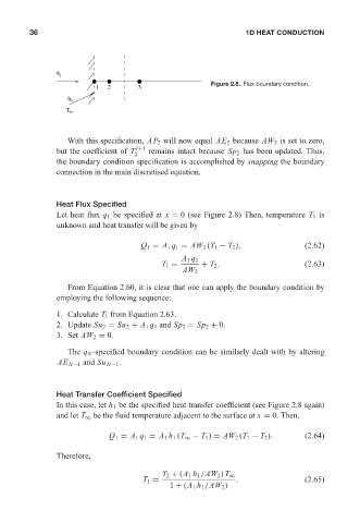
1 2 3 Figure 2.8. Flux boundary condition.
h 1
T 8

With this speciﬁcation, AP 2 will now equal AE 2 because AW 2 is set to zero,
but the coefﬁcient of T 2 l+1 remains intact because Sp 2 has been updated. Thus,
the boundary condition speciﬁcation is accomplished by snapping the boundary
connection in the main discretised equation.

Heat Flux Speciﬁed
Let heat ﬂux q 1 be speciﬁed at x = 0 (see Figure 2.8) Then, temperature T 1 is
unknown and heat transfer will be given by

Q 1 = A 1 q 1 = AW 2 (T 1 − T 2 ), (2.62)
A 1 q 1
T 1 = + T 2 . (2.63)
AW 2

From Equation 2.60, it is clear that one can apply the boundary condition by
employing the following sequence:
1. Calculate T 1 from Equation 2.63.
2. Update Su 2 = Su 2 + A 1 q 1 and Sp 2 = Sp 2 + 0.
3. Set AW 2 = 0.
The q N -speciﬁed boundary condition can be similarly dealt with by altering
AE N−1 and Su N−1 .

Heat Transfer Coefﬁcient Speciﬁed
In this case, let h 1 be the speciﬁed heat transfer coefﬁcient (see Figure 2.8 again)
and let T ∞ be the ﬂuid temperature adjacent to the surface at x = 0. Then,

Q 1 = A 1 q 1 = A 1 h 1 (T ∞ − T 1 ) = AW 2 (T 1 − T 2 ). (2.64)

Therefore,

T 2 + (A 1 h 1 /AW 2 ) T ∞
T 1 = . (2.65)
1 + (A 1 h 1 /AW 2 )

52 53 54 55 56 57 58 59 60 61 62