Page 58 - Introduction to Computational Fluid Dynamics

P1: IWV/ICD
0 521 85326 5
CB908/Date
May 25, 2005
0521853265c02
2.7 DEALING WITH NONLINEARITIES
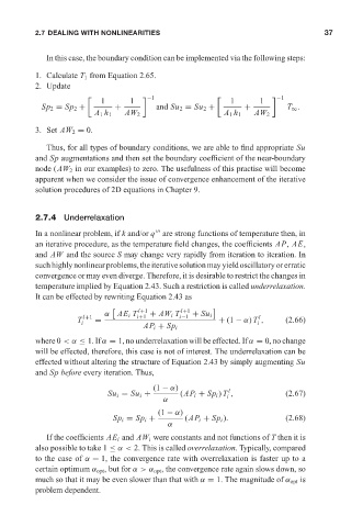
In this case, the boundary condition can be implemented via the following steps: 10:49 37
1. Calculate T 1 from Equation 2.65.
2. Update
1 1 1 1
−1 −1
Sp 2 = Sp 2 + + and Su 2 = Su 2 + + T ∞ .
A 1 h 1 AW 2 A 1 h 1 AW 2
3. Set AW 2 = 0.
Thus, for all types of boundary conditions, we are able to find appropriate Su
and Sp augmentations and then set the boundary coefficient of the near-boundary
node (AW 2 in our examples) to zero. The usefulness of this practise will become
apparent when we consider the issue of convergence enhancement of the iterative
solution procedures of 2D equations in Chapter 9.

2.7.4 Underrelaxation

In a nonlinear problem, if k and/or q are strong functions of temperature then, in
an iterative procedure, as the temperature field changes, the coefficients AP, AE,
and AW and the source S may change very rapidly from iteration to iteration. In
suchhighlynonlinearproblems,theiterativesolutionmayyieldoscillatoryorerratic
convergence or may even diverge. Therefore, it is desirable to restrict the changes in
temperature implied by Equation 2.43. Such a restriction is called underrelaxation.
It can be effected by rewriting Equation 2.43 as

l+1 l+1
α AE i T i+1 + AW i T i−1 + Su i
l
T i l+1 = + (1 − α) T , (2.66)
i
AP i + Sp i
where 0 <α ≤ 1. If α = 1, no underrelaxation will be effected. If α = 0, no change
will be effected, therefore, this case is not of interest. The underrelaxation can be
effected without altering the structure of Equation 2.43 by simply augmenting Su
and Sp before every iteration. Thus,
(1 − α) l
Su i = Su i + (AP i + Sp i ) T , (2.67)
i
α
(1 − α)
Sp i = Sp i + (AP i + Sp i ). (2.68)
α
If the coefficients AE i and AW i were constants and not functions of T then it is
also possible to take 1 ≤ α< 2. This is called overrelaxation. Typically, compared
to the case of α = 1, the convergence rate with overrelaxation is faster up to a
certain optimum α opt , but for α> α opt , the convergence rate again slows down, so
much so that it may be even slower than that with α = 1. The magnitude of α opt is
problem dependent.