Page 62 - Introduction to Computational Fluid Dynamics

P1: IWV/ICD
CB908/Date
0521853265c02
2.8 METHODS OF SOLUTION

Plane Wall 0 521 85326 5 May 25, 2005 10:49 41
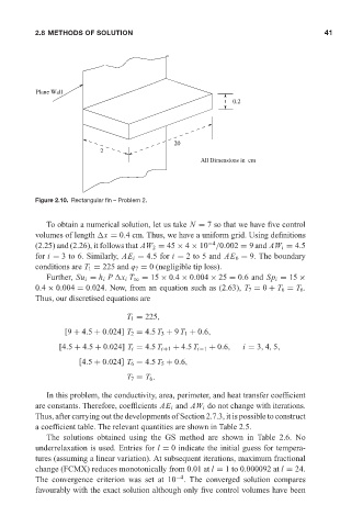
0.2

20
2
All Dimensions in cm

Figure 2.10. Rectangular fin – Problem 2.

To obtain a numerical solution, let us take N = 7 so that we have five control
volumes of length x = 0.4 cm. Thus, we have a uniform grid. Using definitions
−4
(2.25) and (2.26), it follows that AW 2 = 45 × 4 × 10 /0.002 = 9 and AW i = 4.5
for i = 3 to 6. Similarly, AE i = 4.5 for i = 2to5and AE 6 = 9. The boundary
conditions are T 1 = 225 and q 7 = 0 (negligible tip loss).
Further, Su i = h i P x i T ∞ = 15 × 0.4 × 0.004 × 25 = 0.6 and Sp i = 15 ×
0.4 × 0.004 = 0.024. Now, from an equation such as (2.63), T 7 = 0 + T 6 = T 6 .
Thus, our discretised equations are

T 1 = 225,

[9 + 4.5 + 0.024] T 2 = 4.5 T 3 + 9 T 1 + 0.6,
[4.5 + 4.5 + 0.024] T i = 4.5 T i+1 + 4.5 T i−1 + 0.6, i = 3, 4, 5,

[4.5 + 0.024] T 6 = 4.5 T 5 + 0.6,
T 7 = T 6 .

In this problem, the conductivity, area, perimeter, and heat transfer coefficient
are constants. Therefore, coefficients AE i and AW i do not change with iterations.
Thus, after carrying out the developments of Section 2.7.3, it is possible to construct
a coefficient table. The relevant quantities are shown in Table 2.5.
The solutions obtained using the GS method are shown in Table 2.6. No
underrelaxation is used. Entries for l = 0 indicate the initial guess for tempera-
tures (assuming a linear variation). At subsequent iterations, maximum fractional
change (FCMX) reduces monotonically from 0.01 at l = 1 to 0.000092 at l = 24.
−4
The convergence criterion was set at 10 . The converged solution compares
favourably with the exact solution although only five control volumes have been