Page 65 - Introduction to Computational Fluid Dynamics

P1: IWV/ICD
0 521 85326 5
May 25, 2005
10:49
0521853265c02
CB908/Date
44
Table 2.8: Solution by TDMA (N = 8) – Problem 3. 1D HEAT CONDUCTION
x × 10 3 0 2.083 6.25 10.417 14.58 18.75 22.917 25.0
A × 10 5 7.845 7.845 10.5 13.1 15.7 18.3 20.9 23.6
T 200 196.7 192.43 189.4 183.38 177.39 174.63 174.63

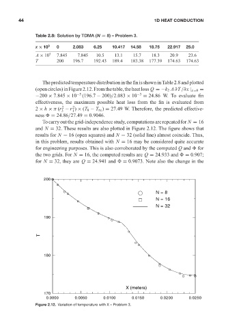
The predicted temperature distribution in the fin is shown in Table 2.8 and plotted
(open circles) in Figure 2.12. From the table, the heat loss Q =−k 2 A ∂T /∂x | x=0 =
−200 × 7.845 × 10 −5 (196.7 − 200)/2.083 × 10 −3 = 24.86 W. To evaluate fin
effectiveness, the maximum possible heat loss from the fin is evaluated from
2
2
2 × h × π (r − r ) × (T 0 − T ∞ ) = 27.49 W. Therefore, the predicted effective-
3
1
ness = 24.86/27.49 = 0.9046.
To carry out the grid-independence study, computations are repeated for N = 16
and N = 32. These results are also plotted in Figure 2.12. The figure shows that
results for N = 16 (open squares) and N = 32 (solid line) almost coincide. Thus,
in this problem, results obtained with N = 16 may be considered quite accurate
for engineering purposes. This is also corroborated by the computed Q and for
the two grids. For N = 16, the computed results are Q = 24.933 and = 0.907;
for N = 32, they are Q = 24.941 and = 0.9073. Note also the change in the

200

N = 8
N = 16
N = 32

190

T

180

X (meters)
170
0.0000 0.0050 0.0100 0.0150 0.0200 0.0250
Figure 2.12. Variation of temperature withX–Problem 3.