Page 70 - Introduction to Computational Fluid Dynamics

P1: IWV/ICD
0 521 85326 5
CB908/Date
0521853265c02
EXERCISES
T 8 May 25, 2005 10:49 49
D
h
B

h i
L

T f
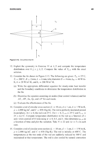
Figure 2.13. Circumferential fin.

12. Exploit the symmetry in Exercise 11 at L/2 and compute the temperature
distribution over 0 ≤ x ≤ L/2. Compare the value of T L/2 with the exact
solution.

◦
13. Consider the fin shown in Figure 2.13. The following are given: T ∞ = 25 C,
T f = 200 C, B = 2 mm, L = 6 mm, tube diameter D = 4 mm, k fin = 40 W/m-
◦
2
2
K, h = 20 W/m -K, and h i = 200 W/m -K.
(a) Write the appropriate differential equation for steady-state heat transfer
and the boundary conditions to determine the temperature distribution in
the fin.
(b) Discretise the equation assuming six nodes (four control volumes) and list
AE, AW, Su, Sp, and AP for each node.
(c) Evaluate the effectiveness of the fin.

14. Consider a rod of circular cross section (L = 10 cm, d = 1 cm, k = 1 W/m-K,
3
ρ = 2,000 kg/m , and C = 850 J/kg-K). The rod is perfectly insulated around
◦ ◦
its periphery. At t = 0, the rod is at 25 C. For t > 0, T x=0 = 25 C and T x=L =
25 + t(s) C. Compute temperature distribution in the rod as a function of x
◦
and t over a period of 15 min using ψ = 0, 0.5, and 1. Also determine q x=0 as
a function of time and plot the variation. Take N = 22 and t = 5 s in each
case.

15. Consider a rod of circular cross section (L = 10 cm, d = 1 cm, k = 1 W/m-K,
3
◦
ρ = 2,000 kg/m , and C = 850 J/kg-K). The rod is initially at 600 C. The
◦
temperatures at the two ends of the rod are suddenly reduced to 100 C and
maintained at that temperature. The rod is also cooled by natural convection