Page 72 - Introduction to Computational Fluid Dynamics

P1: IWV/ICD
0 521 85326 5
CB908/Date
0521853265c02
EXERCISES
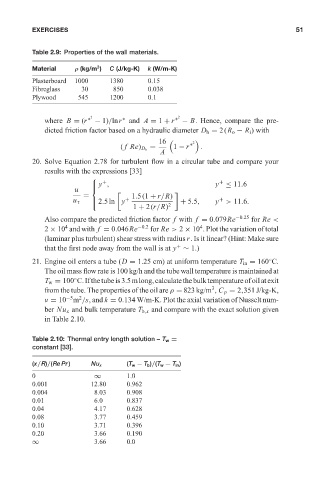
Table 2.9: Properties of the wall materials. May 25, 2005 10:49 51
3
Material ρ (kg/m ) C (J/kg-K) k (W/m-K)
Plasterboard 1000 1380 0.15
Fibreglass 30 850 0.038
Plywood 545 1200 0.1
2 2
∗
where B = (r ∗ − 1)/lnr and A = 1 + r ∗ − B. Hence, compare the pre-
dicted friction factor based on a hydraulic diameter D h = 2(R o − R i ) with
16 2
= 1 − r ∗ .
( fRe) D h
A
20. Solve Equation 2.78 for turbulent flow in a circular tube and compare your
results with the expressions [33]
⎧
+
+
⎪ y , y ≤ 11.6
u ⎨

= 1.5(1 + r/R)
+
⎩ 2.5ln y + + 5.5, y > 11.6.
u τ ⎪
1 + 2(r/R) 2
Also compare the predicted friction factor f with f = 0.079Re −0.25 for Re <
4
4
2 × 10 and with f = 0.046Re −0.2 for Re > 2 × 10 . Plot the variation of total
(laminar plus turbulent) shear stress with radius r. Is it linear? (Hint: Make sure
+
that the first node away from the wall is at y ∼ 1.)
21. Engine oil enters a tube (D = 1.25 cm) at uniform temperature T in = 160 C.
◦
The oil mass flow rate is 100 kg/h and the tube wall temperature is maintained at
T w = 100 C.Ifthetubeis3.5mlong,calculatethebulktemperatureofoilatexit
◦
3
from the tube. The properties of the oil are ρ = 823 kg/m , C p = 2,351 J/kg-K,
2
−5
ν = 10 m /s, and k = 0.134 W/m-K. Plot the axial variation of Nusselt num-
ber Nu x and bulk temperature T b,x and compare with the exact solution given
in Table 2.10.
Table 2.10: Thermal entry length solution – T w =
constant [33].
(x/R)/(Re Pr) Nu x (T w − T b )/(T w − T in )
0 ∞ 1.0
0.001 12.80 0.962
0.004 8.03 0.908
0.01 6.0 0.837
0.04 4.17 0.628
0.08 3.77 0.459
0.10 3.71 0.396
0.20 3.66 0.190
∞ 3.66 0.0