Page 77 - Introduction to Computational Fluid Dynamics

P2: IWV
P1: KsF/ICD/GKJ
10:54
May 25, 2005
0521853265c03
CB908/Date
56
1.0 0 521 85326 5 1D CONDUCTION–CONVECTION
−10
0.8
−4
−2
0.6
P = 0
Φ

0.4 2

4

0.2
10

0.0
0.00 0.25 0.50 0.75 1.00
X
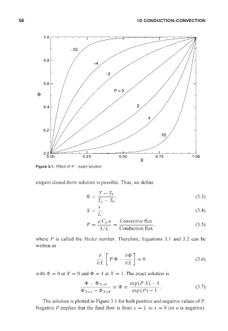
Figure 3.1. Effect of P – exact solution.

elegant closed-form solution is possible. Thus, we define

T − T 0
= , (3.3)
T L − T 0
x
X = , (3.4)
L
ρ C p u Convective flux
P = = , (3.5)
k/L Conduction flux

where P is called the Peclet number. Therefore, Equations 3.1 and 3.2 can be
written as

∂ ∂
P − = 0 (3.6)
∂ X ∂ X

with = 0at X = 0 and = 1at X = 1. The exact solution is

− X=0 exp (PX) − 1
= = . (3.7)
X=1 − X=0 exp (P) − 1
The solution is plotted in Figure 3.1 for both positive and negative values of P.
Negative P implies that the fluid flow is from x = L to x = 0 (or u is negative).