Page 78 - Introduction to Computational Fluid Dynamics

P2: IWV
P1: KsF/ICD/GKJ
CB908/Date
0 521 85326 5
0521853265c03
May 25, 2005
3.3 DISCRETISATION
It will be instructive to note the tendencies exhibited by the solution. 10:54 57
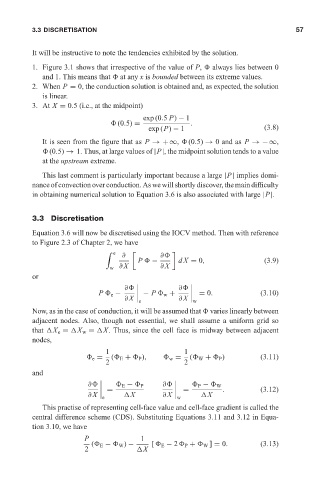
1. Figure 3.1 shows that irrespective of the value of P, always lies between 0
and 1. This means that at any x is bounded between its extreme values.
2. When P = 0, the conduction solution is obtained and, as expected, the solution
is linear.
3. At X = 0.5 (i.e., at the midpoint)
exp (0.5 P) − 1
(0.5) = .
exp (P) − 1 (3.8)
It is seen from the figure that as P →+∞, (0.5) → 0 and as P →−∞,
(0.5) → 1. Thus, at large values of |P|, the midpoint solution tends to a value
at the upstream extreme.

This last comment is particularly important because a large |P| implies domi-
nance of convection over conduction. As we will shortly discover, the main difficulty
in obtaining numerical solution to Equation 3.6 is also associated with large |P|.

3.3 Discretisation
Equation 3.6 will now be discretised using the IOCV method. Then with reference
to Figure 2.3 of Chapter 2, we have
e
∂ ∂
P − dX = 0, (3.9)
w ∂ X ∂ X
or

∂ ∂
P e − − P w + = 0. (3.10)
∂ X e ∂ X w
Now, as in the case of conduction, it will be assumed that varies linearly between
adjacent nodes. Also, though not essential, we shall assume a uniform grid so
that X e = X w = X. Thus, since the cell face is midway between adjacent
nodes,
1 1
e = ( E + P ), w = ( W + P ) (3.11)
2 2
and

∂ E − P ∂ P − W
= = . (3.12)
∂ X e X ∂ X w X
This practise of representing cell-face value and cell-face gradient is called the
central difference scheme (CDS). Substituting Equations 3.11 and 3.12 in Equa-
tion 3.10, we have

P 1
( E − W ) − [ E − 2 P + W ] = 0. (3.13)
2 X