Page 81 - Introduction to Computational Fluid Dynamics

P2: IWV
P1: KsF/ICD/GKJ
10:54
May 25, 2005
0 521 85326 5
CB908/Date
0521853265c03
60
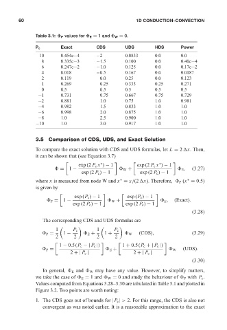
Table 3.1: Φ P values for Φ E = 1 and Φ W = 0. 1D CONDUCTION–CONVECTION
Exact CDS UDS HDS Power
P c
10 0.454e−4 −2 0.0833 0.0 0.0
8 0.335e−3 −1.5 0.100 0.0 0.40e−4
6 0.247e−2 −1.0 0.125 0.0 0.17e−2
4 0.018 −0.5 0.167 0.0 0.0187
2 0.119 0.0 0.25 0.0 0.123
1 0.269 0.25 0.333 0.25 0.271
0 0.5 0.5 0.5 0.5 0.5
−1 0.731 0.75 0.667 0.75 0.729
−2 0.881 1.0 0.75 1.0 0.981
−4 0.982 1.5 0.833 1.0 1.0
−6 0.998 2.0 0.875 1.0 1.0
−8 1.0 2.5 0.900 1.0 1.0
−10 1.0 3.0 0.917 1.0 1.0

3.5 Comparison of CDS, UDS, and Exact Solution
To compare the exact solution with CDS and UDS formulas, let L = 2 x. Then,
it can be shown that (see Equation 3.7)
exp (2 P c x ) − 1 exp (2 P c x ) − 1
∗ ∗
= 1 − W + E , (3.27)
exp (2 P c ) − 1 exp (2 P c ) − 1
where x is measured from node W and x = x/(2 x). Therefore, P (x = 0.5)
∗
∗
is given by

exp (P c ) − 1 exp (P c ) − 1
P = 1 − W + E , (Exact).
exp (2 P c ) − 1 exp (2 P c ) − 1
(3.28)
The corresponding CDS and UDS formulas are
1 P c 1 P c
P = 1 − E + 1 + W (CDS), (3.29)
2 2 2 2

1 − 0.5(P c −| P c |) 1 + 0.5(P c +| P c |)
P = E + W (UDS).
2 +| P c | 2 +| P c |
(3.30)
In general, E and W may have any value. However, to simplify matters,
we take the case of E = 1 and W = 0 and study the behaviour of P with P c .
Values computed from Equations 3.28–3.30 are tabulated in Table 3.1 and plotted in
Figure 3.2. Two points are worth noting:

1. The CDS goes out of bounds for |P c | > 2. For this range, the CDS is also not
convergent as was noted earlier. It is a reasonable approximation to the exact