Page 86 - Introduction to Computational Fluid Dynamics

P2: IWV
P1: KsF/ICD/GKJ
0 521 85326 5
0521853265c03
CB908/Date
3.9 STABILITY OF THE UNSTEADY EQUATION
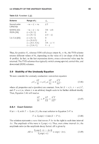
Table 3.2: Function f c (ξ). May 25, 2005 10:54 65
Scheme Range of ξ f c
Second-order −∞ <ξ < ∞ ξ/2
UPWIND
QUICK [42] −∞ <ξ < ∞ 3/8 − ξ/4
HLPA [90] ξ [0, 1] 0
ξ ∈ [0, 1] ξ (1 − ξ)
Lin–Lin [43] ξ [0, 1] 0
ξ ∈ [0, 0.3] ξ
ξ ∈ [0.3, 5/6] 3/8 − ξ /4
ξ ∈ [5/6, 1] 1 − ξ

Thus, for positive P c , whereas UDS will always return e = P , the TVD scheme
returns different values of e depending on the value of ξ (or shape of the local
profile). In fact, as the last expression shows, even a downwind value may be
returned. The TVD schemes thus typically switch among upwind, central-like, and
downwind (DDS) schemes.

3.9 Stability of the Unsteady Equation

We now consider the unsteady conduction–convection equation
2
∂T ∂T ∂ T
ρ C p + ρ C p u = k 2 , (3.46)
∂t ∂x ∂x
2
where all properties and u (positive) are constant. Now, let X = x/λ, τ = α t/λ ,
and P = u λ/α, where λ is an arbitrary length scale to be further defined shortly.
Then, Equation 3.46 will read as
2
∂T ∂T ∂ T
+ P = . (3.47)
∂τ ∂ X ∂ X 2

3.9.1 Exact Solution
If at t = 0, with T = T 0 sin (X ), the exact solution to Equation 3.47 is

T = T 0 exp(−τ)sin(X − P τ). (3.48)

The solution represents a wave that moves P τ to the right in each time interval
τ. The amplitude of the wave is T 0 exp(−τ). Thus, over a time interval τ, the
amplitude ratio (or the amplitude decay factor) AR is given by

T 0 exp [−(τ + τ)]
AR = = exp(− τ). (3.49)
T 0 exp(−τ)