Page 88 - Introduction to Computational Fluid Dynamics

P2: IWV
P1: KsF/ICD/GKJ
0 521 85326 5
0521853265c03
CB908/Date
3.9 STABILITY OF THE UNSTEADY EQUATION
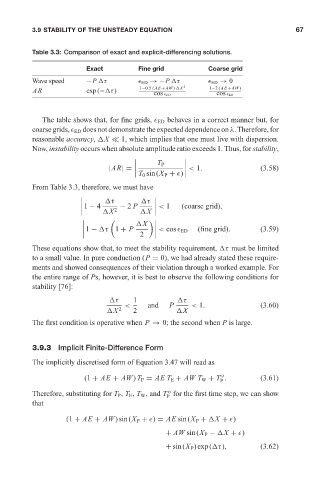
Table 3.3: Comparison of exact and explicit-differencing solutions. May 25, 2005 10:54 67
Exact Fine grid Coarse grid
Wave speed −P τ ED →−P τ ED → 0
1−0.5(AE+AW) X 2 1−2(AE+AW)
AR exp(− τ)
cos ED cos ED
The table shows that, for fine grids, ED behaves in a correct manner but, for
coarse grids, ED does not demonstrate the expected dependence on λ. Therefore, for
reasonable accuracy, X 1, which implies that one must live with dispersion.
Now, instability occurs when absolute amplitude ratio exceeds 1. Thus, for stability,

T P
|AR|= < 1. (3.58)
T 0 sin(X P + )
From Table 3.3, therefore, we must have

τ
τ
1 − 4 − 2 P < 1 (coarse grid),

X 2 X

X
1 − τ 1 + P (3.59)
< cos ED (fine grid).
2
These equations show that, to meet the stability requirement, τ must be limited
to a small value. In pure conduction (P = 0), we had already stated these require-
ments and showed consequences of their violation through a worked example. For
the entire range of Ps, however, it is best to observe the following conditions for
stability [76]:
τ 1 τ
< and P < 1. (3.60)
X 2 2 X
The first condition is operative when P → 0; the second when P is large.

3.9.3 Implicit Finite-Difference Form

The implicitly discretised form of Equation 3.47 will read as
o
(1 + AE + AW) T P = AE T E + AW T W + T . (3.61)
P
o
Therefore, substituting for T P , T E , T W , and T for the first time step, we can show
P
that
(1 + AE + AW)sin(X P + ) = AE sin(X P + X + )
+ AW sin(X P − X + )

+ sin(X P )exp( τ), (3.62)