Page 93 - Introduction to Computational Fluid Dynamics

P1: IWV
CB908/Date
0 521 85326 5
0521853265c04
May 25, 2005
72
2D BOUNDARY LAYERS
E Boundary 11:7
y
Boundary Layer
Axisymmetric Body
I Boundary
x r I r

α Axis of Symmetry
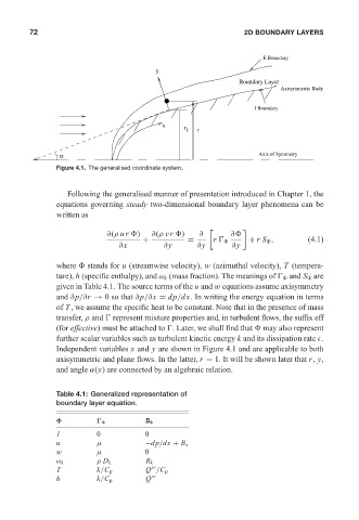
Figure 4.1. The generalised coordinate system.

Following the generalised manner of presentation introduced in Chapter 1, the
equations governing steady two-dimensional boundary layer phenomena can be
written as

∂(ρ ur ) ∂(ρv r ) ∂ ∂
+ = r
+ rS , (4.1)
∂x ∂y ∂y ∂y

where stands for u (streamwise velocity), w (azimuthal velocity), T (tempera-
ture), h (specific enthalpy), and ω k (mass fraction). The meanings of
and S are
given in Table 4.1. The source terms of the u and w equations assume axisymmetry
and ∂p/∂r → 0 so that ∂p/∂x = dp/dx. In writing the energy equation in terms
of T , we assume the specific heat to be constant. Note that in the presence of mass
transfer, ρ and
represent mixture properties and, in turbulent flows, the suffix eff
(for effective) must be attached to
. Later, we shall find that may also represent
further scalar variables such as turbulent kinetic energy k and its dissipation rate .
Independent variables x and y are shown in Figure 4.1 and are applicable to both
axisymmetric and plane flows. In the latter, r = 1. It will be shown later that r, y,
and angle α(x) are connected by an algebraic relation.

Table 4.1: Generalized representation of
boundary layer equation.
Φ Γ Φ S Φ

1 0 0
u µ −dp/dx + B x
w µ 0
ω k ρ D k R k

T k/C p Q /C p
h k/C p Q