Page 94 - Introduction to Computational Fluid Dynamics

P1: IWV
CB908/Date
0 521 85326 5
0521853265c04
4.2 ADAPTIVE GRID
Wasted Nodes May 25, 2005 11:7 73
y max E Boundary

ω
y
x x
I Boundary
Too Fine Too Coarse
(a) (b)
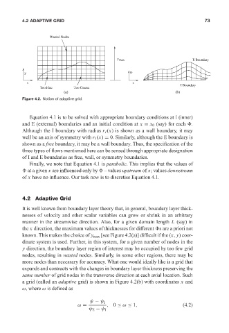
Figure 4.2. Notion of adaptive grid.

Equation 4.1 is to be solved with appropriate boundary conditions at I (inner)
and E (external) boundaries and an initial condition at x = x 0 (say) for each .
Although the I boundary with radius r I (x) is shown as a wall boundary, it may
well be an axis of symmetry with r I (x) = 0. Similarly, although the E boundary is
shown as a free boundary, it may be a wall boundary. Thus, the specification of the
three types of flows mentioned here can be sensed through appropriate designation
of I and E boundaries as free, wall, or symmetry boundaries.
Finally, we note that Equation 4.1 is parabolic. This implies that the values of
atagiven x are influenced only by – values upstream of x; values downstream
of x have no influence. Our task now is to discretise Equation 4.1.

4.2 Adaptive Grid
It is well known from boundary layer theory that, in general, boundary layer thick-
nesses of velocity and other scalar variables can grow or shrink in an arbitrary
manner in the streamwise direction. Also, for a given domain length L (say) in
the x direction, the maximum values of thicknesses for different s are a priori not
known. This makes the choice of y max [see Figure 4.2(a)] difficult if the (x, y) coor-
dinate system is used. Further, in this system, for a given number of nodes in the
y direction, the boundary layer region of interest may be occupied by too few grid
nodes, resulting in wasted nodes. Similarly, in some other regions, there may be
more nodes than necessary for accuracy. What one would ideally like is a grid that
expands and contracts with the changes in boundary layer thickness preserving the
same number of grid nodes in the transverse direction at each axial location. Such
a grid (called an adaptive grid) is shown in Figure 4.2(b) with coordinates x and
ω, where ω is defined as

ψ − ψ I
ω = , 0 ≤ ω ≤ 1, (4.2)
ψ E − ψ I