Page 98 - Introduction to Computational Fluid Dynamics

P1: IWV
CB908/Date
0 521 85326 5
0521853265c04
4.4 DISCRETISATION
Xu Xd May 25, 2005 11:7 77
E Boundary (j = JN)
j = JN − 1
N j + 1
n

P j ∆ω
P
s
S j − 1

ω
j = 2
I Boundary (j = 1)
x

∆x
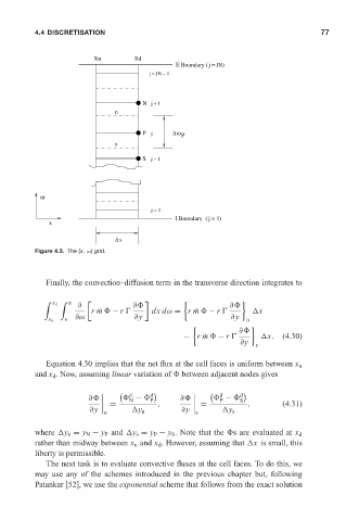
Figure 4.3. The (x, ω) grid.

Finally, the convection–diffusion term in the transverse direction integrates to

n
∂ ∂ ∂
x d
r ˙ m − r
dx dω = r ˙ m − r
x
∂ω ∂y ∂y
s
x u n
∂

− r ˙ m − r
x. (4.30)
∂y
s
Equation 4.30 implies that the net flux at the cell faces is uniform between x u
and x d . Now, assuming linear variation of between adjacent nodes gives

− −
d d d d
∂ N P ∂ P S
= , = , (4.31)
∂y ∂y
n y n s y s
where y n = y N − y P and y s = y P − y S . Note that the s are evaluated at x d
rather than midway between x u and x d . However, assuming that x is small, this
liberty is permissible.
The next task is to evaluate convective fluxes at the cell faces. To do this, we
may use any of the schemes introduced in the previous chapter but, following
Patankar [52], we use the exponential scheme that follows from the exact solution