Page 60 - Introduction to Computational Fluid Dynamics

P1: IWV/ICD
CB908/Date
0521853265c02
2.8 METHODS OF SOLUTION
6
2 3 4 0 521 85326 5 7 8 9 10 N − 1 May 25, 2005 10:49 39
5
2 1 −a
2 0 0 0 0 0 0 0 0 T C
2 2
3 −b
3 1 −a 0 0 0 0 0 0 0 T C
3 3 3
4 0 0 0 0 0 0 0
0 0 0 0 0
5 0 0
6 0 0 0 0 − b i 1 − a i 0 0 0 0 T C
i i
0
7 00 0 00 0 0 0 0
0 0 0 0
8 0 0 0
9 0 0 0 0 0 0 0

0 0 − a
10 0 0 0 0 0 10
N − 1 0 0 00 0 0 0 0 0 0 0 −b N−1 1 T N−1 C N−1

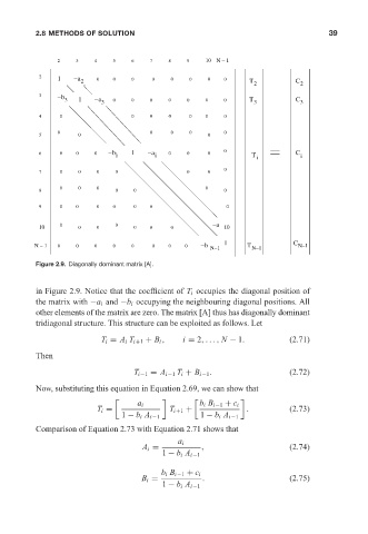
Figure 2.9. Diagonally dominant matrix [A].

in Figure 2.9. Notice that the coefficient of T i occupies the diagonal position of
the matrix with −a i and −b i occupying the neighbouring diagonal positions. All
other elements of the matrix are zero. The matrix [A] thus has diagonally dominant
tridiagonal structure. This structure can be exploited as follows. Let
T i = A i T i+1 + B i , i = 2,..., N − 1. (2.71)

Then

T i−1 = A i−1 T i + B i−1 . (2.72)
Now, substituting this equation in Equation 2.69, we can show that

a i b i B i−1 + c i
T i = T i+1 + . (2.73)
1 − b i A i−1 1 − b i A i−1
Comparison of Equation 2.73 with Equation 2.71 shows that
a i
A i = , (2.74)
1 − b i A i−1

b i B i−1 + c i
B i = . (2.75)
1 − b i A i−1