Page 64 - Introduction to Computational Fluid Dynamics

P1: IWV/ICD
0 521 85326 5
CB908/Date
0521853265c02
2.8 METHODS OF SOLUTION
Table 2.7: Solution by TDMA – Problem 2. May 25, 2005 10:49 43
x (cm) 0 0.2 0.6 1.0 1.4 1.8 2
A i − 0.333 0.598 0.711 0.772 0.0 −
B i − 149.78 89.628 63.776 49.357 212.375 −
l = 1 225 222.45 218.40 215.38 213.37 212.37 212.37
Exact 225 222.58 218.52 215.51 213.49 212.49 212.37

2
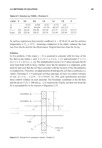
fin surface experiences heat transfer coefficient h = 20 W/m -K and the ambient
◦
temperature is T ∞ = 25 C. Assuming conduction to be radial, estimate the heat
loss from the fin and the fin effectiveness. Neglect heat loss from the fin tip.

Solution
In this problem, if the origin x = 0 is assumed to coincide with the base of the
fin, then at any radius r, area A = 2π rt = 2π (r 1 + x)t and perimeter P = 2 ×
(2π r) = 2 × [2π (r 1 + x)]. The multiplication factor 2 in P arises because the fin
loses heat from both its faces. Further, since the fin material is a composite, grids
must be laid such that the cell face coincides with the location of the discontinuity
in conductivity. Therefore, we adopt practise B and specify cell-face coordinate (x c )
values. Choosing N = 8 and equal cell-face spacings, we have six control volumes
of size x = (r 3 − r 1 )/(N − 2) = 0.4167 cm. This grid specification provides
three control volumes in each material. The boundary conditions at the fin base
and fin tip are T (1) = 200 and q N = 0, respectively. Finally, the heat loss from the
fin is accounted for in the manner of Equations 2.51.

MATERIAL K 3

r 3
MATERIAL K
2
r 2
r
T 0 1

TUBE

h
ANNULAR
Τ 8
FIN
t
Figure 2.11. Annular fin of composite material – Problem 3.