Page 48 - Introduction to Computational Fluid Dynamics

P1: IWV/ICD
0 521 85326 5
CB908/Date
0521853265c02
2.5 STABILITY AND CONVERGENCE
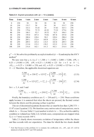
Table 2.1: Explicit procedure with ∆t = 10 s (stable). May 25, 2005 10:49 27
Time 0 mm 1 mm 3 mm 5 mm 7 mm 9 mm 10 mm
0 250 30 30 30 30 30 250
10 250 135.7 30 30 30 135.7 250
20 250 165.3 55.43 30 55.43 165.3 250
30 250 179.6 75.72 42.22 75.22 179.6 250
40 250 188.5 92.5 58.33 92.5 188.5 250
50 250 195.0 107.4 74.82 107.4 195.0 250
60 250 200.4 120.6 90.5 120.6 200.4 250
70 250 205.1 132.6 105.0 132.6 205.1 250
80 250 209.3 143.4 118.3 143.4 209.3 250
90 250 213.0 153.2 130.3 153.2 213.0 250
100 250 216.4 162.1 141.3 162.1 216.4 250

q = 0. We solve this problem by an explicit method (ψ = 0) and employ the IOCV

method. 5
We now note that ρ A i x i C = 1,300 × 1 × 0.002 × 2,000 = 5,200, AW 2 =
0.25 × 1/0.001 = 250, AW i = 0.25 × 1/0.002 = 125 for i = 3to N − 1,
AE N−1 = 0.25 × 1/0.001 = 250, and AE i = 0.25 × 1/0.002 = 125 for i = 2to
N − 2. Therefore, the applicable discretised equations are

5,200 o o 5,200 o
T 2 = 250 T + 125 T + − 375 T , (2.33)
1
2
3
t t
5,200
o o 5,200 o
T i = 125 T + T + − 250 T , (2.34)
t i−1 i+1 t i
for i = 3, 4, and 5 and
5,200 o o 5,200 o
T N−1 = 125 T N−2 + 250 T + − 375 T N−1 . (2.35)
N
t t
Finally, the boundary conditions are T 1 = 250 and T N = 250. These conditions
apply because it is assumed that when the sheets are pressed, the thermal contact
between the sheets and the pressing surface is perfect.
This set of discretised equations dictates that t must be less than 5,200/375 =
13.87 s (see Equation 2.32). We therefore carry out two sets of computations, one in
which t = 10 s (see Table 2.1) and another in which t = 20 s, so that the stability
condition is violated (see Table 2.2). In both cases, computations are stopped when
◦
T 4 (x = 5 mm) exceeds 140 C.
Table 2.1 clearly shows monotonic evolution of temperature within the sheets
and thus accords with our expectation. The time for which the two sheets should

5 Note that because in this problem kA is constant, the coefficients AE i , AW i , and AP i will be
identical in both the IOCV and TSE methods.