Page 40 - Introduction to Computational Fluid Dynamics

P1: IWV/ICD
CB908/Date
0 521 85326 5
0521853265c02
2.3 GRID LAYOUT
PRACTISE A May 25, 2005 10:49 19
Xc 1,2 3 4 5 6 7 8 9

X 12 3 4 5 6 7 8
N = 9

PRACTISE B
CELL FACE
1,2 3 4 5 6 7 8 9

12 3 4 5 6 7 8N = 9
NODE
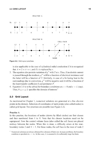
Figure 2.2. Grid layout practises.

is also applicable to the case of cylindrical radial conduction if it is recognised
that A = 2 × π × r, and if x is replaced by r.
3. The equation also permits variation of q with T or x. Thus, if an electric current

is passed through the medium, q will be a function of electrical resistance and

the latter will be a function of T. Similarly, in case of a fin losing heat to the
surroundings due to convection, q will be negative and it will be a function of

the heat transfer coefficient h and perimeter P.
4. Equation 2.5 is to be solved for boundary conditions at x = 0 and x = L (say).
Thus, 0 ≤ x ≤ L specifies the domain of interest. 1

2.3 Grid Layout

As mentioned in Chapter 1, numerical solutions are generated at a few discrete
points in the domain. Selection of coordinates of such points (also called nodes) is
called grid layout. Two practises are possible (see Figure 2.2).

Practise A
In this practise, the locations of nodes (shown by filled circles) are first chosen
and then numbered from 1 to N. Note that the chosen locations need not be
equispaced. Now the control volume faces (also called the cell faces) are placed
midway between the nodes. When this is done, a difficulty arises at the near-
boundary nodes 2 and N − 1. For these nodes, the cell face to the west of node 2

1 Numerical solutions are always obtained for a domain of finite size. In many problems, the boundary
condition is specified at x =∞. In this case, L is assumed to be sufficiently large but finite.