Page 116 - Introduction to chemical reaction engineering and kinetics

98 Chapter 5: Complex Systems

from which kf can be determined from measured values of fA (or cA) at various times
t , if Kc,eq is known. Then k, is obtained from
kr = kflKc,,, (5.3-19)

If the reaction is allowed to reach equilibrium (t + m), Kc,eq can be calculated from

K c,eq = ‘D,eq Geq (5.3-20)
lc
0 gression of equation 5.3-18 to obtain kf (or a corresponding linear graph), a nonlin-
As an alternative to this traditional procedure, which involves, in effect, linear re-
v
ear regression procedure can be combined with simultaneous numerical integration of
“O-v
equation 5.3-17a. Results of both these procedures are illustrated in Example 5-4. If the
reaction is carried out at other temperatures, the Arrhenius equation can be applied to
each rate constant to determine corresponding values of the Arrhenius parameters.

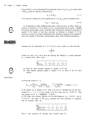
Assuming that the isomerization of A to D and its reverse reaction are both first-order:

calculate the values of kf and k, from the following data obtained at a certain temperature
in a constant-volume batch reactor: 0 1 2 3 4m

t/h
v
45.6
72.5 56.8
100cAIcAo
100
39.5 30
“OF
0 (a) Using the linear procedure indicated in equation 5.3-18; and
(b) Using nonlinear regression applied to equation 5.3-17 by means of the E-Z Solve
software.
SOLUTION

(a) From the result at t = a~,

K c&J - ‘De _ CAofA,,eq 1 - CA,eq’CAo = 0.7/0.3 = 2 . 3 3
‘Aeq cAo(1 - fA,,eq) = ‘A,t?qIcAo

In the simplest use of equation 5.3-18, values of kf may be calculated from the four mea-
surements at t = 1, 2, 3, 4 h; the average of the four values gives kf = 0.346 h-l. Then,
from equation 5.3-19, k, = 0.346/2.33 = 0.148 h-t.
(b) The results from nonlinear regression (see file ex5-4.msp) are: kf = 0.345 h-l and kf
= 0.147 h-‘. The values of 100 cAIcA~ calculated from these parameters, in comparison
with the measured values are:

t/h 1 2 3 4
(~OOCAICA~)~~~ 72.5 56.8 45.6 39.5 3:
UOOCAICA~~ 72.8 56.1 45.9 39.7 29.9

There is close agreement, the (absolute) mean deviation being 0.3.