Page 249 - Introduction to chemical reaction engineering and kinetics

9.1 Gas-Solid (Reactant) Systems 231

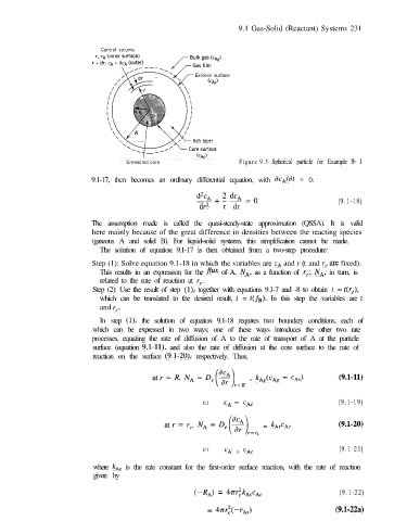
Control volume

Exterior surface

Unreacted core Figure 9.3 Spherical particle for Example 9- 1

9.1-17, then becomes an ordinary differential equation, with dc,ldt = 0:
d2cA (9.1-18)
-+2dc,=()
dr2 r dr

The assumption made is called the quasi-steady-state approximation (QSSA). It is valid
here mainly because of the great difference in densities between the reacting species
(gaseous A and solid B). For liquid-solid systems, this simplification cannot be made.
The solution of equation 9.1-17 is then obtained from a two-step procedure:

Step (1): Solve equation 9.1-18 in which the variables are cA and r (t and r, are fixed).
This results in an expression for the flux of A, NA, as a function of r,; NA, in turn, is
related to the rate of reaction at r,.
Step (2): Use the result of step (l), together with equations 9.1-7 and -8 to obtain t = t(r,),
which can be translated to the desired result, t = t(&). In this step the variables are t
and rC.
In step (l), the solution of equation 9.1-18 requires two boundary conditions, each of
which can be expressed in two ways; one of these ways introduces the other two rate
processes, equating the rate of diffusion of A to the rate of transport of A at the particle
surface (equation 9.1-ll), and also the rate of diffusion at the core surface to the rate of
reaction on the surface (9.1-20), respectively. Thus,

= k&+, - cAs)

o r CA = ch (9.1-19)

= kAsCAc

o r (9.1-21)
cA = cAc
where kAs is the rate constant for the first-order surface reaction, with the rate of reaction
given by

(-RA) = 4TrzkAsCAc (9.1-22)

= 47Trz(-rh) (9.1-22a)