Page 187 - Materials Chemistry, Second Edition

9.3 Methodology 185
The global weight of a criterion was determined by the crisp local weight multiplying the
crisp perspective weight, as shown in Eq. (9.5).

w global ¼ w perspective w local (9.5)

9.3.4 Step 4. Rank the alternatives by the goal programming method

The goal programming method is a classical scheduling method (Papathanasiou and
Ploskas, 2018). The goal programming has been revised to be adapted in problem selection
by limiting the assigned alternative as one. In this case study, the goal programming method
was adapted to select the best option among three oil management systems.
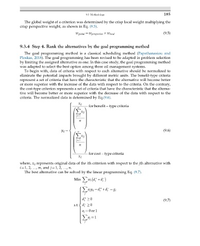
To begin with, data of criteria with respect to each alternative should be normalized to
eliminate the potential impacts brought by different metric units. The benefit-type criteria
represent a set of criteria that have the characteristic that the alternative will become better
or more superior with the increase of the data with respect to the criteria. On the contrary,
the cost-type criterion represents a set of criteria that have the characteristic that the alterna-
tive will become better or more superior with the decrease of the data with respect to the
criteria. The normalized data is determined by Eq.(9.6).
8
x ij
>
> 1 for benefit type criteria
> 0 n
> X
>
>
> x ij
> B C
>
>
> B j¼1 C
>
> B C
>
> B n C
>
> @ A
>
>
>
<
y ij ¼ 0 n 1 (9.6)
> X
>
> x ij
>
> B C
>
> B j¼1 C
>
> B C
>
> B n C
>
> @ A
>
>
>
>
>
> for cost type criteria
>
:
x ij
where, x ij represents original data of the ith criterion with respect to the jth alternative with
i¼1, 2, …, m, and j¼1, 2, …, n.
The best alternative can be solved by the linear programming Eq. (9.7).
X +
Min w i d + d
i
i
i
8 X
+
> a j y ij d + d ¼ g i
i
i
>
>
> j
>
>
>
> +
> d 0
> i (9.7)
>
<
s:t: d 0

i
>
>
> a j ¼ 0or1
>
>
>
> X
>
> a j ¼ 1
>
>
:
j