Page 154 - MATLAB an introduction with applications

Control Systems ——— 139

y = lsim (num, den, r, t) ...(3.66)
y = lsim (A, B, C, D, u, t) ...(3.67)
The MATLAB commands in Eqs. (3.64) to (3.67) will generate the response to input time function r or u

3.21 RESPONSE TO INITIAL CONDITION IN STATE SPACE

Consider the system defined in state space by
x = Ax + Bu, x (0) = x 0 ...(3.68)
y = Cx + Du ...(3.69)
The MATLAB command
initial (A, B, C, D, [initial condition], t) ...(3.70)
may be used to provide the response to the initial condition.

3.22 EXAMPLE PROBLEMS AND SOLUTIONS

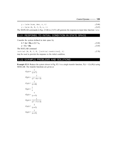
Example E3.1: Reduce the system shown in Fig. E3.1 to a single transfer function, T(s) = C(s)/R(s) using
MATLAB. The transfer functions are given as
1
G (s) = (s + 7)
1
1
G (s) = (s + 6s + 5)
2
2
1
G (s) = (s + 8)
3
1
G (s) = s
4
7
G (s) = (s + 3)
5
1
G (s) = (s + 7s + 5)
6
2
5
G (s) = (s + 5)
7
1
G (s) = (s + 9)
8

F:\Final Book\Sanjay\IIIrd Printout\Dt. 10-03-09