Page 158 - MATLAB an introduction with applications

Control Systems ——— 143

>> omeganc=sqrt(denc(3))
omeganc = 3.1623e+004
>> zetac=denc (2)/(2*omeganc)
zetac = 0.2095
>> Tsc = 4/ (zetac*omeganc)
Tsc = 6.0377e-004
>> Tpc =pi/ (omeganc*sqrt (1–zetac^2))
Tpc = 1.0160e-004
>> Trc = (1.76*zetac^3 –.417*zetac^2 + 1.039*zetac + 1)/ omeganc
Trc = 3.8439e-005
>> percentc =exp (–zetac*pi/ sqrt (1–zetac^2))*100
percentc = 51.0123
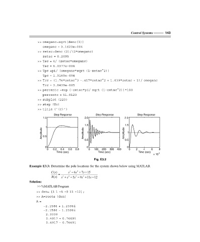
>> subplot (223)
>> step (Tc)
>> title (‘(c)’)

Step Response Step Response Step Response
1.5 2.0 2.0
1.5 1.5
1
Amplitude 0.5 Amplitude 1 Amplitude 1

0.5 0.5

0 0 0
0 0.2 0.4 0.6 0.8 0 100 200 300 400 0 2 4 6 8
Time (sec) Time (sec) Time (sec)
× 10 4
Fig. E3.2
Example E3.3: Determine the pole locations for the system shown below using MATLAB.
2
()
Cs = s − 6s + 7s + 15
3
()
Rs s + s − 5s − 9s + 11s − 12
5
4
2
3
Solution:
>> %MATLAB Program
>> den= [1 1 –5 –9 11 –12];
>> A=roots (den)
A =
–2.1586 + 1.2396i
–2.1586 – 1.2396i
2.3339
0.4917 + 0.7669i
0.4917 – 0.7669i

F:\Final Book\Sanjay\IIIrd Printout\Dt. 10-03-09