Page 160 - MATLAB an introduction with applications

Control Systems ——— 145

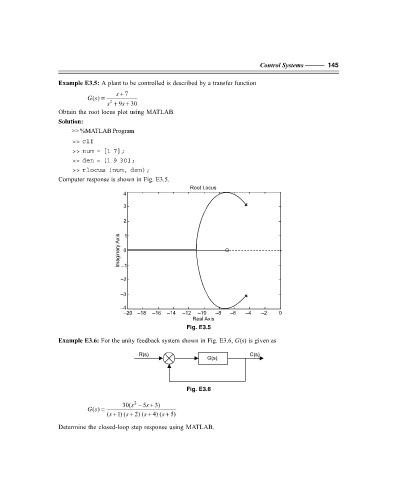
Example E3.5: A plant to be controlled is described by a transfer function
s + 7
() =
Gs
s + 9s + 30
2
Obtain the root locus plot using MATLAB.
Solution:
>> %MATLAB Program
>> clf
>> num = [1 7];
>> den = [1 9 30];
>> rlocus (num, den);
Computer response is shown in Fig. E3.5.
Root Locus
4
3

2

Imaginary Axis 0 1

–1
–2

–3
–4
–20 –18 –16 –14 –12 –10 –8 –6 –4 –2 0
Real Axis
Fig. E3.5
Example E3.6: For the unity feedback system shown in Fig. E3.6, G(s) is given as

R(s) C(s)
G(s)

Fig. E3.6
2
30(s − 5s + 3)
() =
Gs
(s + 1) (s + 2) (s + 4) (s + 5)
Determine the closed-loop step response using MATLAB.

F:\Final Book\Sanjay\IIIrd Printout\Dt. 10-03-09