Page 156 - MATLAB an introduction with applications

Control Systems ——— 141

Inputs = 9;
Outputs = 7;
Ts = connect (T1, Q, Inputs, Outputs);
T = Tf (Ts) computer response
Transfer function:
10 s^7 + 290 s^6 + 3350 s^5 + 1.98e004 s^4 + 6.369e004 s^3 + 1.089e005 s^2
+ 8.895e004 s + 2.7e004 s^10 + 45 s^9 + 866 s^8 + 9305 s^7 + 6.116e004 s^6 +
2.533e005 s^5 + 6.57e005 s^4 + 1.027e006 s^3 + 8.909e005 s^2 + 3.626e005 s
+ 4.2e004
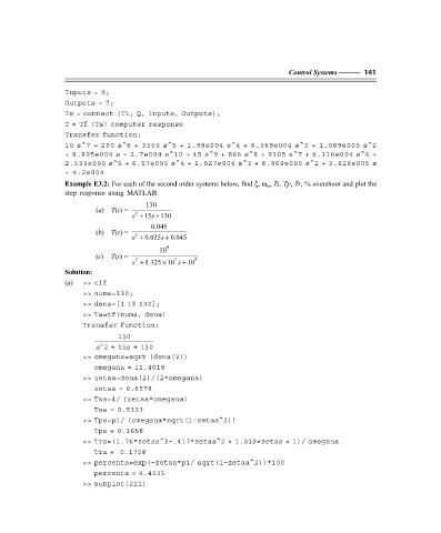
Example E3.2: For each of the second order systems below, find ξ, ω , Ts, Tp, Tr, % overshoot and plot the
n
step response using MATLAB.
130
(a) T(s) =
s + 15s + 130
2
0.045
(b) T(s) =
2
s + 0.025s + 0.045
10 8
(c) T(s) =
×
2
s + 1.325 10 s + 10 8
3
Solution:
(a) >> clf
>> numa=130;
>> dena=[1 15 130];
>> Ta=tf(numa, dena)
Transfer function:
130
s ∧ 2 + 15s + 130
>> omegana=sqrt (dena(3))
omegana = 11.4018
>> zetaa=dena(2)/(2*omegana)
zetaa = 0.6578
>> Tsa=4/ (zetaa*omegana)
Tsa = 0.5333
>> Tpa=pi/ (omegana*sqrt(1–zetaa^2))
Tpa = 0.3658
>> Tra=(1.76*zetaa^3–.417*zetaa^2 + 1.039*zetaa + 1)/ omegana
Tra = 0.1758
>> percenta=exp(–zetaa*pi/ sqrt(1–zetaa^2))*100
percenta = 6.4335
>> subplot(221)

F:\Final Book\Sanjay\IIIrd Printout\Dt. 10-03-09