Page 252 - MATLAB an introduction with applications

Numerical Methods ——— 237

X = X0;
[L,U] = lu(P);
fprintf(‘iter#\tX(1)\t\tX(2)\n’);
while er>tole & k<kstop
fprintf(‘%d\t%f\t%f\n’,k,X(1),X(2));
k = k+1;
dx = L\r;
dx = U\dx;
X = X+dx;
r = b–A*X;
er = norm(r)/r0;
erp(k) = norm(r)/r0;
end
X
plot(erp, ‘–p’);
grid on;
xlabel(‘Iteration #’);
ylabel(‘normalized error’);

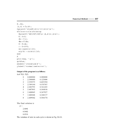
Output of the program is as follows:
iter# X(1) X(2)
0 0.000000 0.000000
1 2.500000 0.125000
2 2.359375 0.433594
3 2.389160 0.535767
4 2.403793 0.561245
5 2.407893 0.566810
6 2.408845 0.567927
7 2.409044 0.568137
8 2.409082 0.568174

The final solution is
X =
2.4091
0.5682
0.9318
The variation of error in each cycle is shown in Fig. E4.16.