Page 253 - MATLAB an introduction with applications
P. 253

238 ———  MATLAB: An Introduction with Applications


                                       0.14

                                       0.12

                                        0.1
                                      error  0.08
                                      Normalized  0.06


                                       0.04

                                       0.02

                                         0
                                          1     2    3     4    5     6    7     8    9
                                                             Iteration #
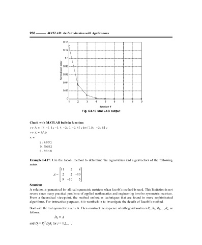
                                                   Fig. E4.16 MATLAB output


                   Check with MATLAB built-in function:
                   >> A = [4 –1 1;–1 4 –2;1 –2 4];b=[10; –2;5];
                   >> x = A\b
                   x =
                         2.4091
                          0.5682
                         0.9318

                   Example E4.17: Use the Jacobi method to determine the eigenvalues and eigenvectors of the following
                   matrix
                                      11   2    8
                                     
                                                  
                                 A =  2     2 –10
                                     
                                                  
                                        9 –10  5 
                   Solution:
                   A solution is guaranteed for all real symmetric matrices when Jacobi’s method is used. This limitation is not
                   severe since many practical problems of applied mathematics and engineering involve symmetric matrices.
                   From a theoretical viewpoint, the method embodies techniques that are found in more sophisticated
                   algorithms. For instructive purposes, it is worthwhile to investigate the details of Jacobi’s method.

                   Start with the real symmetric matrix A. Then construct the sequence of orthogonal matrices R , R , R ,…,R   as
                                                                                                 3
                                                                                                      n
                                                                                           1
                                                                                              2
                   follows:
                                    D =  A
                                   0
                            T
                   and D = R D R  for j = 1,2,...  .
                        j
                              j j
                           j
   248   249   250   251   252   253   254   255   256   257   258