Page 325 - MATLAB an introduction with applications

310 ——— MATLAB: An Introduction with Applications

Iteration 2:

∇ f 2
2
U = –∇f + 1 U 1
1
∇ f 0 2
2
2
1
2
X = X + λ U and perform line search to find the minimum of f(X ) = f(λ )
2
2
Again compute ∇f (X ). Stop if it is equal to zero otherwise continue.
2
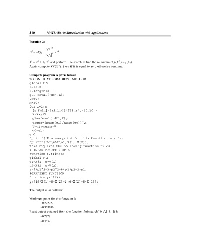
Complete program is given below:
% CONJUGATE GRADIENT METHOD
global X V
X=[0;0];
N=length(X);
g0=–feval(‘df’,X);
V=g0;
n=50;
for i=1:n
[s fmin]=fminbnd(‘fline’,–10,10);
X=X+s*V
g1=–feval(‘df’,X);
gamma=(norm(g1)/norm(g0))^2;
V=g1+gamma*V;
g0=g1;
end
fprintf(‘Minimum point for this function is \n’);
fprintf(‘%f\n%f\n’,X(1),X(2));
This requires the following function files
%LINEAR FUNCTION OF s
function z=fline(s)
global V X
p1=X(1)+s*V(1);
p2=X(2)+s*V(2);
z=9*p1^2+3*p2^2–8*p1*p2+2*p1;
%GRADIENT FUNCTION
function y=df(X)
y=[18*X(1)–8*X(2)+2;6*X(2)–8*X(1)];

The output is as follows:

Minimum point for this function is
–0.272727
–0.363636
Exact output obtained from the function fminsearch(‘fxy’,[–1,1]) is
–0.2727
–0.3637