Page 321 - MATLAB an introduction with applications

306 ——— MATLAB: An Introduction with Applications

2 2
2
Example E5.26: Find the minimum of the function f = 90(y – x ) + (1 – x) with Powell’s method starting at
the point (–1, 1).
Solution:

() =
Let X be an initial guess at the location of the minimum of the function z = f X f x x 2 ..., ) . Assume
( , ,
x
n
0
1
that the partial derivatives of the function are not available. An intuitively appealing approach to

approximating a minimum of the function f is to generate the next approximation X by proceeding
1
successively to a minimum of f along each of the n standard base vectors. This process can be called
the taxi-cab method and generates the sequence of points

X 0 = P 0, P P 2..., P = X 1
1,
n

Along each standard base vector E = (0,...0,1 ,0,...,0) the function f is a function of one variable, and
k
k
the minimization of f might be accomplished by the application of either the golden ratio or Fibonacci
searches if f is unimodal in this search direction. The iteration is then repeated to generate a sequence of

}
points{X k k= 0 . Unfortunately, the method is, in general, inefficient due to the geometry of multivariable
functions.
1  0 
Choose N =2 and select two direction vectors U =  and U = .
2 
1
1
0
 
−  1  −+ 1 
1 λ
Start with point P = X =   and construct P = P + λ U =   by moving P 1
1
1
0
1
0
 1   1  X 2 =P 2
in the directions U by optimal length λ . Substituting P in f, a one-dimensional
1
1
1
objective function is formed in λ , which is solved for minimum. Then λ is U
1
1
substituted in P and new point P is evaluated as P = P +λ U by moving in P 0 =X U
2
2
1
2
1
2
P 1
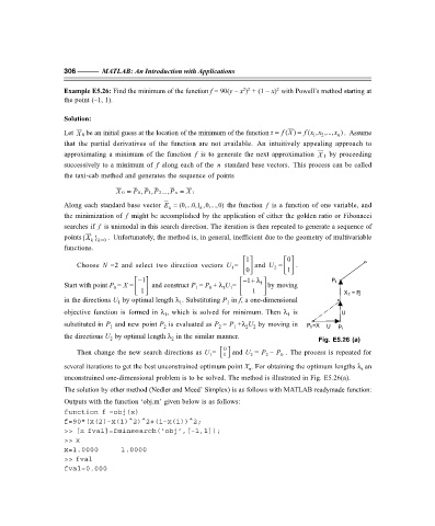
the directions U by optimal length λ in the similar manner. Fig. E5.26 (a)
2
2
0
Then change the new search directions as U =  and U = P – P . The process is repeated for
1 
0
1
2
2
several iterations to get the best unconstrained optimum point X . For obtaining the optimum lengths λ an
n
i
unconstrained one-dimensional problem is to be solved. The method is illustrated in Fig. E5.26(a).
The solution by other method (Nedler and Meed’ Simplex) is as follows with MATLAB readymade function:
Outputs with the function ‘obj.m’ given below is as follows:
function f =obj(x)
f=90*(x(2)–x(1)^2)^2+(1–x(1))^2;
>> [x fval]=fminsearch(‘obj’,[–1,1]);
>> x
x=1.0000 1.0000
>> fval
fval=0.000